Processing lidar and UAV point clouds in GRASS GIS (workshop at FOSS4G Boston 2017): Difference between revisions
⚠️Wenzeslaus (talk | contribs) |
⚠️Wenzeslaus (talk | contribs) No edit summary |
||
| Line 2: | Line 2: | ||
[[File:Grassgis logo colorlogo text whitebg.png|400px|right|none]] | [[File:Grassgis logo colorlogo text whitebg.png|400px|right|none]] | ||
Description: GRASS GIS offers, besides other things, numerous analytical tools for point clouds, terrain, and remote sensing. In this hands-on workshop we will explore the tools in GRASS GIS for processing point clouds obtained by lidar or through processing of UAV imagery. We will start with a brief and focused introduction into GRASS GIS graphical user interface (GUI) and we will continue with short introduction to GRASS GIS Python interface. Participants will then decide if they will use GUI, command line, Python, or online Jupyter Notebook for the rest of the workshop. We will explore the properties of the point cloud, interpolate surfaces, and perform advanced terrain analyses to detect landforms and artifacts. We will go through several terrain 2D and 3D visualization techniques to get more information out of the data and finish with vegetation analysis. | |||
Requirements: This workshop is accessible to beginners, but some basic knowledge of lidar processing or GIS is helpful for a smooth experience. | Requirements: This workshop is accessible to beginners, but some basic knowledge of lidar processing or GIS is helpful for a smooth experience. | ||
Revision as of 13:27, 18 July 2017
Description: GRASS GIS offers, besides other things, numerous analytical tools for point clouds, terrain, and remote sensing. In this hands-on workshop we will explore the tools in GRASS GIS for processing point clouds obtained by lidar or through processing of UAV imagery. We will start with a brief and focused introduction into GRASS GIS graphical user interface (GUI) and we will continue with short introduction to GRASS GIS Python interface. Participants will then decide if they will use GUI, command line, Python, or online Jupyter Notebook for the rest of the workshop. We will explore the properties of the point cloud, interpolate surfaces, and perform advanced terrain analyses to detect landforms and artifacts. We will go through several terrain 2D and 3D visualization techniques to get more information out of the data and finish with vegetation analysis.
Requirements: This workshop is accessible to beginners, but some basic knowledge of lidar processing or GIS is helpful for a smooth experience.
Authors: Vaclav Petras, Anna Petrasova, and Helena Mitasova from North Carolina State University
Preparation
Software
GRASS GIS 7.2 compiled with libLAS is needed (e.g. r.in.lidar should work).
OSGeo-Live
All needed software is included.
Ubuntu
Install GRASS GIS from packages:
sudo add-apt-repository ppa:ubuntugis/ubuntugis-unstable
sudo apt-get update
sudo apt-get install grass
Linux
For other Linux distributions other then Ubuntu, please try to find GRASS GIS in their package managers.
MS Windows
Download the standalone GRASS GIS binaries from grass.osgeo.org.
Mac OS
Install GRASS GIS using Homebrew osgeo4mac:
brew tap osgeo/osgeo4mac
brew install grass7
Note that currently (summer 2017) r.in.lidar is often not accessible on Mac OS, use r.in.ascii in combination with libLAS or PDAL command line tools to achieve the same. Note also that the 3D view may not be accessible.
Data
Basic introduction to graphical user interface
Basic introduction to Python interface
The simplest way to execute the Python code which uses GRASS GIS packages is to use Simple Python editor integrated in GRASS GIS (accessible from the toolbar or the Python tab in the Layer Manager). Another option is to write the Python code in your favorite plain text editor like Notepad++ (note that Python editors are plain text editors). Then run the script in GRASS GIS using the main menu File -> Launch script.
-
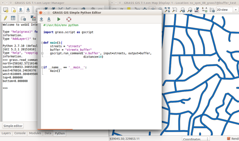
Simple Python Editor integrated in GRASS GIS (since version 7.2) with Python tab in the background which contains an interactive Python shell.
-
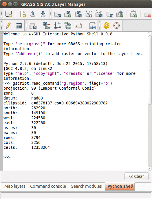
Python tab with an interactive Python shell


The GRASS GIS 7 Python Scripting Library provides functions to call GRASS modules within scripts as subprocesses. The most often used functions include:
- script.core.run_command(): used with modules which output raster/vector data where text output is not expected
- script.core.read_command(): used when we are interested in text output
- script.core.parse_command(): used with modules producing text output as key=value pair
- script.core.write_command(): for modules expecting text input from either standard input or file
We will use GRASS GUI Simple Python Editor to run the commands. You can open it from Python tab. For longer scripts, you can create a text file, save it into your current working directory and run it with python myscript.py from the GUI command console or terminal.
When you open Simple Python Editor, you find a short code snippet. It starts with importing GRASS GIS Python Scripting Library:
import grass.script as gscript
In the main function we call g.region to see the current computational region settings:
gscript.run_command('g.region', flags='p')
Note that the syntax is similar to bash syntax (g.region -p), only the flag is specified in a parameter. Now we can run the script by pressing the Run button in the toolbar. In Layer Manager we get the output of g.region.
Before running any GRASS raster modules, you need to set the computational region. In this example, we set the computational extent and resolution to the raster layer elevation. Replace the previous g.region command with the following line:
gscript.run_command('g.region', raster='dsm')
The run_command() function is the most commonly used one. We will use it to compute viewshed using r.viewshed. Add the following line after g.region command:
gscript.run_command('r.viewshed', input='dsm', output='python_viewshed', coordinates=(640645, 224035), overwrite=True)
Parameter overwrite is needed if we rerun the script and rewrite the raster.
Now let's look at how big the viewshed is by using
r.univar. Here we use parse_command to obtain the statistics as a Python dictionary
univar = gscript.parse_command('r.univar', map='python_viewshed', flags='g')
print univar['n']
The printed result is the number of cells of the viewshed.
GRASS GIS Python Scripting Library also provides several wrapper functions for often called modules. List of convenient wrapper functions with examples includes:
- Raster metadata using script.raster.raster_info():
gscript.raster_info('viewshed_python') - Vector metadata using script.vector.vector_info():
gscript.vector_info('roads') - List raster data in current location using script.core.list_grouped():
gscript.list_grouped(type=['raster']) - Get current computational region using script.core.region():
gscript.region()
Here are two commands (to be executed in the Console) often used when working with scripts. First is setting the computational region. We can do that in a script, but it is better and more general to do it before executing the script (so that the script can be used with different computational region settings):
g.region raster=dsm
The second command is handy when we want to run the script again and again. In that case, we first need to remove the created raster maps, for example:
g.remove type=raster pattern="viewshed*"
The above command actually won't remove the maps, but it will inform you which it will remove if you provide the -f flag.
Decide if to use GUI, command line, Python, or online Jupyter Notebook
Binning of the point cloud
Compute density of point cloud:
 g.region  n=224034 s=223266 e=640086 w=639318 res=1
 r.in.lidar -o input=tile_0793_016_spm.las method=n output=tile_density_1m resolution=1
 r.in.lidar -o input=tile_0793_016_spm.las method=n output=tile_density_6m resolution=6
We can use binning to compute the range of elevation values and other statistics:
 r.in.lidar -o input=tile_0793_016_spm.las method=range output=tile_range_6m resolution=6
 # the map and the following statistics show there is an outlier at around 600 m
 r.report map=tile_range_6m units=c
 # change the color table to histogram equalized to see the contrast
 r.colors map=tile_range_6m color=viridis -e
We can filter data by class or return:
 r.in.lidar -o input=tile_0793_016_spm.las method=mean output=tile_ground_6m resolution=6 class_filter=2
 r.colors map=tile_ground_6m color=elevation
Interpolation
First we import LAS file as vector points, we keep only first return points and limit the import vertically to avoid using outliers found in the previous step.
v.in.lidar -obt input=tile_0793_016_spm.las output=tile_points return_filter=first zrange=0,300
Then we interpolate:
 g.region -a -p vector=tile_points res=2
 v.surf.rst input=tile_points elevation=tile_dsm tension=25 smooth=1 npmin=100
Now you can visualize the resulting DSM using 3D view (first uncheck all other layers and then switch to 3D) or by computing shaded relief with r.relief.
Terrain analysis
Visualization, profiles and statistics
Vegetation analysis
3D visualization

We can explore our study area in 3D view (use image on the right if clarification is needed for below steps):
- Add raster dsm and uncheck or remove any other layers. Any layer in Layer Manager is interpreted as surface in 3D view.
- Switch to 3D view (in the right corner of Map Display).
- Adjust the view (perspective, height).
- In Data tab, set Fine mode resolution to 1 and set ortho as the color of the surface (the orthophoto is draped over the DSM).
- Go back to View tab and explore the different view directions using the green puck.
- Go again to Data tab and change color to viewshed raster computed in the previous steps.
- Go to Appearance tab and change the light conditions (lower the light height, change directions).
- When finished, switch back to 2D view.