Processing lidar and UAV point clouds in GRASS GIS (workshop at FOSS4G Boston 2017)
Description: GRASS GIS offers, besides other things, numerous analytical tools for point clouds, terrain, and remote sensing. In this hands-on workshop we will explore the tools in GRASS GIS for processing point clouds obtained by lidar or through processing of UAV imagery. We will start with a brief and focused introduction into GRASS GIS graphical user interface (GUI) and we will continue with short introduction to GRASS GIS Python interface. Participants will then decide if they will use GUI, command line, Python, or online Jupyter Notebook for the rest of the workshop. We will explore the properties of the point cloud, interpolate surfaces, and perform advanced terrain analyses to detect landforms and artifacts. We will go through several terrain 2D and 3D visualization techniques to get more information out of the data and finish with vegetation analysis.
Requirements: This workshop is accessible to beginners, but some basic knowledge of lidar processing or GIS is helpful for a smooth experience.
Authors: Vaclav Petras, Anna Petrasova, and Helena Mitasova from North Carolina State University
Contributors: Robert S. Dzur and Doug Newcomb
Testers:
Preparation
Software
GRASS GIS 7.2 compiled with libLAS is needed (e.g. r.in.lidar should work).
OSGeo-Live
All needed software is included.
Ubuntu
Install GRASS GIS from packages:
sudo add-apt-repository ppa:ubuntugis/ubuntugis-unstable
sudo apt-get update
sudo apt-get install grass
Linux
For other Linux distributions other then Ubuntu, please try to find GRASS GIS in their package managers.
MS Windows
Download the standalone GRASS GIS binaries from grass.osgeo.org.
Mac OS
Install GRASS GIS using Homebrew osgeo4mac:
brew tap osgeo/osgeo4mac
brew install grass7
Note that currently (summer 2017) r.in.lidar is often not accessible on Mac OS, use r.in.ascii in combination with libLAS or PDAL command line tools to achieve the same. Note also that the 3D view may not be accessible.
Addons
You will need to install the following GRASS GIS Addons. This can be done through GUI, but for simplicity copy and paste and execute the following lines one by one in the command line:
g.extension r.geomorphon
g.extension r.skyview
g.extension r.local.relief
g.extension r.shaded.pca
g.extension r.area
g.extension r.terrain.texture
g.extension r.fill.gaps
For bonus tasks:
g.extension v.lidar.mcc
Data
Basic introduction to graphical user interface
GRASS GIS Spatial Database
Here we provide an overview of GRASS GIS. For this exercise it's not necessary to have a full understanding of how to use GRASS GIS. However, you will need to know how to place your data in the correct GRASS GIS database directory, as well as some basic GRASS functionality.
GRASS uses specific database terminology and structure (GRASS GIS Spatial Database) that are important to understand for working in GRASS GIS efficiently. You will create a new location and import the required data into that location. In the following we review important terminology and give step by step directions on how to download and place your data in the correct place.
- A GRASS GIS Spatial Database (GRASS database) consists of directory with specific Locations (projects) where data (data layers/maps) are stored.
- Location is a directory with data related to one geographic location or a project. All data within one Location has the same coordinate reference system.
- Mapset is a collection of maps within Location, containing data related to a specific task, user or a smaller project.
Start GRASS GIS, a start-up screen should appear. Unless you already have a directory called grassdata in your Documents directory (on MS Windows) or in your home directory (on Linux), create one. You can use the Browse button and the dialog in the GRASS GIS start up screen to do that.
We will create a new location for our project with CRS (coordinate reference system) NC State Plane Meters with EPSG code 3358. Open Location Wizard with button New in the left part of the welcome screen. Select a name for the new location, select EPSG method and code 3358. When the wizard is finished, the new location will be listed on the start-up screen. Select the new location and mapset PERMANENT and press Start GRASS session.
-
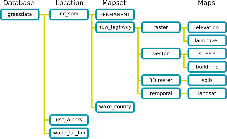
GRASS GIS Spatial Database structure
-
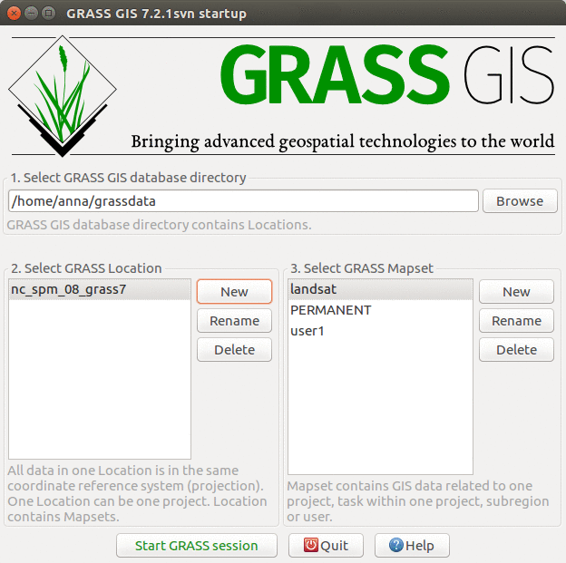
GRASS GIS 7.2 startup dialog
-
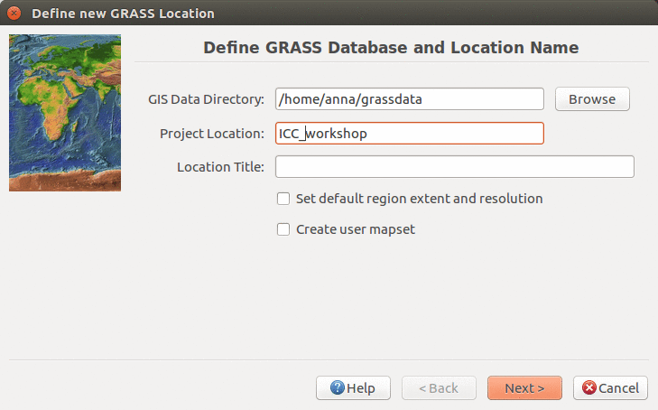
Start Location Wizard and type the new location's name
-
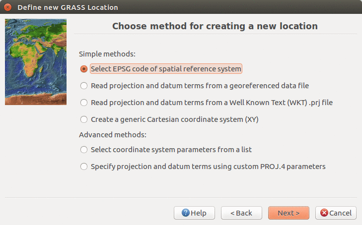
Select method for describing CRS
-
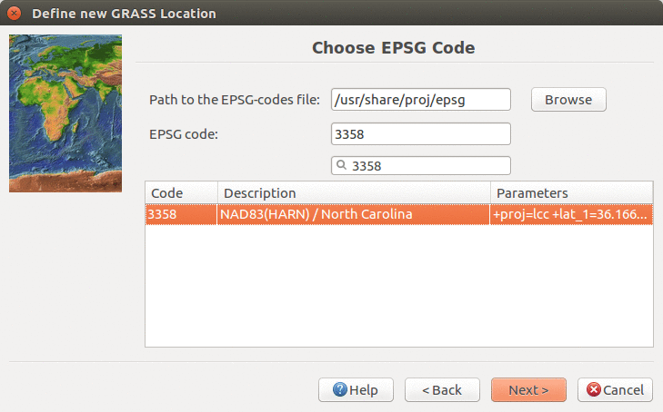
Find and select EPSG 3358
-
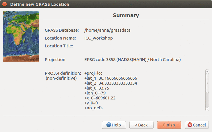
Review summary page and confirm


Note that a current working directory is a concept which is separate from the GRASS database, location and mapset discussed above. The current working directory is a directory where any program (no just GRASS GIS) writes and reads files unless a path to the file is provided. The current working directory can be changed from the GUI using Settings → GRASS working environment → Change working directory or from the Console using the cd command.
Importing data
In this step we import the provided data into GRASS GIS. In menu File - Import raster data select Common formats import and in the dialog browse to find ortho.tif and click button Import. All the imported layers should be added to GUI automatically, if not, add them manually. Point clouds will be imported later in a different way as part of the analysis.
-
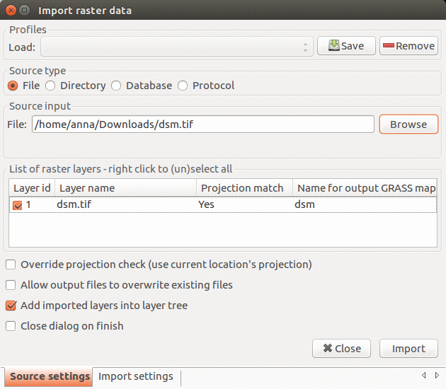
Import raster data

Computational region
Before we use a module to compute a new raster map, we must properly set the computational region. All raster computations will be performed in the specified extent and with the given resolution.
Computational region is an important raster concept in GRASS GIS. In GRASS a computational region can be set, subsetting larger extent data for quicker testing of analysis or analysis of specific regions based on administrative units. We provide a few points to keep in mind when using the computational region function:
- defined by region extent and raster resolution
- applies to all raster operations
- persists between GRASS sessions, can be different for different mapsets
- advantages: keeps your results consistent, avoid clipping, for computationally demanding tasks set region to smaller extent, check that your result is good and then set the computational region to the entire study area and rerun analysis
- run
g.region -por in menu Settings - Region - Display region to see current region settings
-
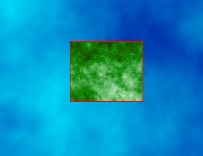
Computational region concept: A raster with large extent (blue) is displayed as well as another raster with smaller extent (green). The computational region (red) is now set to match the smaller raster, so all the computations are limited to the smaller raster extent even if the input is the larger raster. (Not shown on the image: Also the resolution, not only the extent, matches the resolution of the smaller raster.)
-
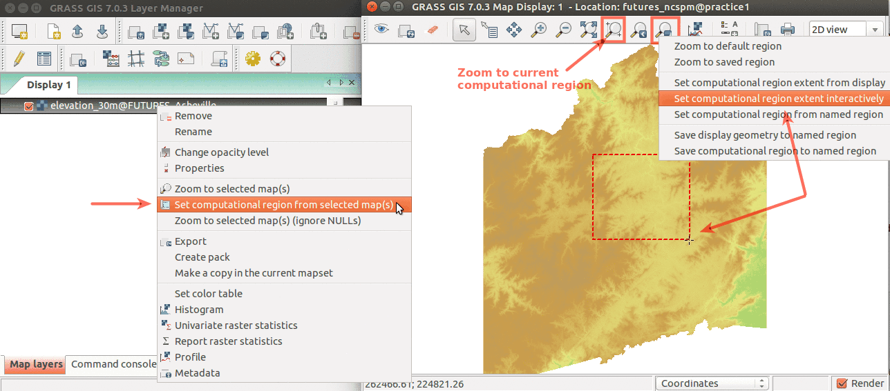
Simple ways to set computational region from GUI: On the left, set region to match raster map. On the right, select the highlighted option and then set region by drawing rectangle.
-
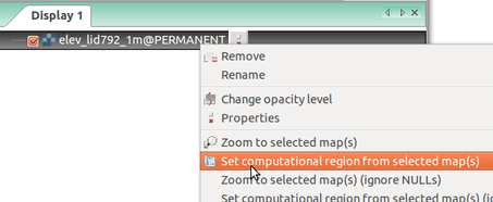
Set computational region (extent and resolution) to match a raster (Layers tab in the Layer Manager)


The numeric values of computational region can be checked using:
g.region -p
After executing the command you will get something like this:
north:      220750
south:      220000
west:       638300
east:       639000
nsres:      1
ewres:      1
rows:       750
cols:       700
cells:      525000
Computational region can be set using a raster map:
g.region raster=ortho -p
Resolution can be set separately using the res parameter of the g.region module. The units are the units of the current location, in our case meters. This can be done in the Resolution tab of the g.region dialog or in the command line in the following way (using also the -a flag to print the new values):
g.region res=3 -p
The new resolution may be slightly modified in this case to fit into the extent which we are not changing. However, often we want the resolution to be the exact value we provide and we are fine with a slight modification of the extent. That's what -a flag is for. On the other hand, if alignment with cells of a specific raster is important, align parameter can be used to request the alignment to that raster (regardless of the the extent).
The following example command will use the extent from the raster named ortho, use resolution 5 meters, modify the extent to align it to this 5 meter resolution, and print the values of this new computational region settings:
g.region vector=ortho res=5 -a -p
Modules
GRASS GIS functionality is available through modules (tools, functions, commands). Modules respect the following naming conventions:
| Prefix | Function | Example |
|---|---|---|
| r. | raster processing | r.mapcalc: map algebra |
| v. | vector processing | v.surf.rst: surface interpolation |
| i. | imagery processing | i.segment: image segmentation |
| r3. | 3D raster processing | r3.stats: 3D raster statistics |
| t. | temporal data processing | t.rast.aggregate: temporal aggregation |
| g. | general data management | g.remove: removes maps |
| d. | display | d.rast: display raster map |
These are the main groups of modules. There is few more for specific purposes. Note also that some modules have multiple dots in their names. This often suggests further grouping. For example, modules staring with v.net. deal with vector network analysis. The name of the module helps to understand its function, for example v.in.lidar starts with v so it deals with vector maps, the name follows with in which indicates that the module is for importing the data into GRASS GIS Spatial Database and finally lidar indicates that it deals with lidar point clouds.
-
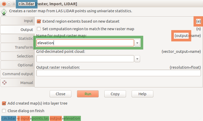
r.in.lidar dialog with Output tab active and highlighted module name (blue), options and flags (red) and option values (green)
-
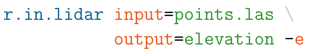
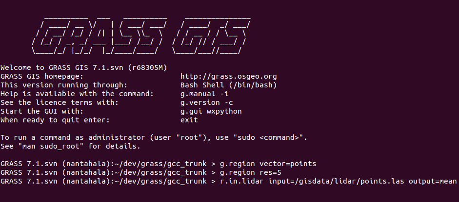
Example r.in.lidar command in Bash with highlighted module name (blue), options and flags (red) and option values (green)
-
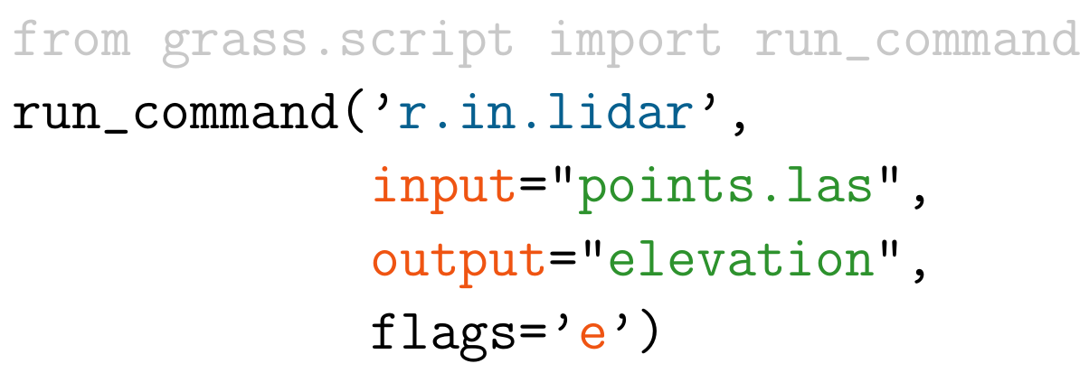
Example r.in.lidar command in Python with highlighted module name (blue), options and flags (red) and option values (green) and import (grey)
-
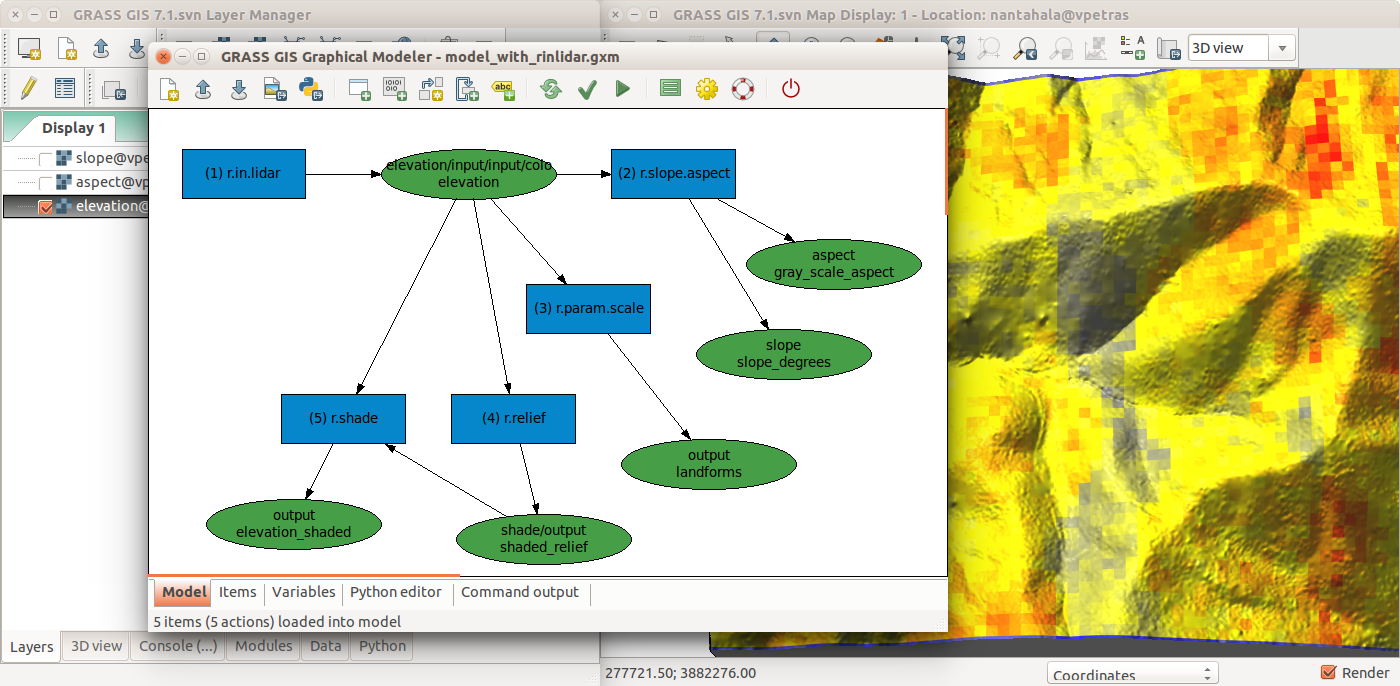
GRASS GIS Graphical Modeler
-
Console tab in the Layer Manager for running commands or opening module dialogs
-
Command line interface (CLI) in a system terminal
-
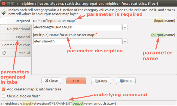
Layout of a module dialog
-
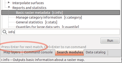
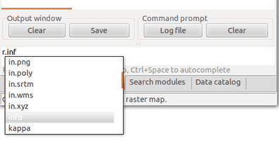
Search for a module in the Modules tab


One of the advantages of GRASS GIS is the diversity and number of modules that let you analyze all manners of spatial and temporal data. GRASS GIS has over 500 different modules in the core distribution and over 300 addon modules that can be used to prepare and analyze data. The following table lists some of the main modules for point cloud analysis.
| Module | Function | Alternatives |
|---|---|---|
| r.in.lidar | binning into 2D raster, statistics | r.in.xyz, v.vect.stats, r.vect.stats |
| v.in.lidar | import, decimation | v.in.ascii, v.in.ogr, v.import |
| r3.in.lidar | binning into 3D raster | r3.in.xyz |
| v.out.lidar | export of point cloud | v.out.ascii, r.out.xyz |
| v.surf.rst | interpolation surfaces from points | v.surf.bspline, v.surf.idw |
| v.lidar.edgedetection | ground and object (edge) detection | v.lidar.mcc, v.outlier |
| v.decimate | decimate (thin) a point cloud | v.in.lidar, r.in.lidar |
| r.slope.aspect | topographic parameters | v.surf.rst |
| r.relief | shaded relief computation | r.skyview |
| r.colors | raster color table management | r.cpt2grass, r.colors.matplotlib |
| g.region | resolution and extent management | r.in.lidar, GUI |
Basic introduction to Python interface
The simplest way to execute the Python code which uses GRASS GIS packages is to use Simple Python Editor integrated in GRASS GIS (accessible from the toolbar or the Python tab in the Layer Manager). Another option is to use your favorite text editor and then run the script in GRASS GIS using the main menu File → Launch script.
-
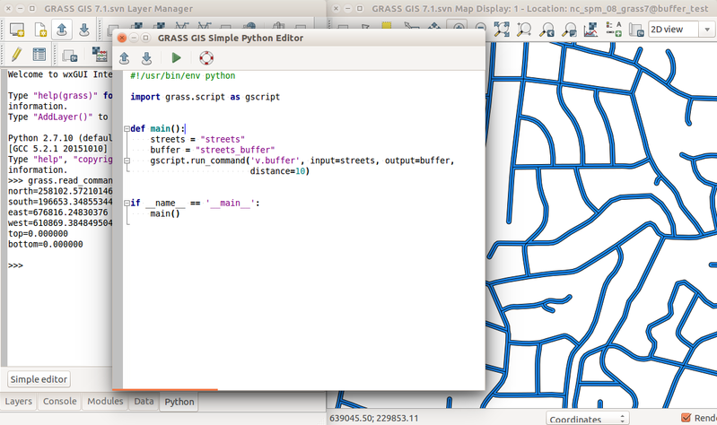
Simple Python Editor integrated in GRASS GIS
-
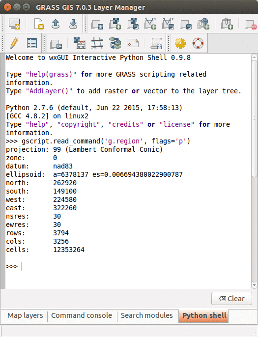
Python tab with an interactive Python shell


The GRASS GIS 7 Python Scripting Library provides functions to call GRASS modules within Python scripts as subprocesses. All functions are in a package called grass and the most common functions are in grass.script package which is often imported import grass.script as gscript. The most often used functions include:
- script.core.run_command(): used with modules which output raster or vector data and when text output is not expected
- script.core.read_command(): used when we are interested in text output which is returned as Python string
- script.core.parse_command(): used with modules producing text output as key=value pair which is automatically parsed into a Python dictionary
- script.core.write_command(): for modules expecting text input from either standard input or file
We will use the Simple Python Editor to run the commands. You can open it from the Python tab.
When you open Simple Python Editor, you find a short code snippet. It starts with importing GRASS GIS Python Scripting Library:
import grass.script as gscript
In the main function we call g.region to see the current computational region settings:
gscript.run_command('g.region', flags='p')
Note that the syntax is similar to bash syntax (g.region -p), only the flag is specified in a parameter. Now we can run the script by pressing the Run button in the toolbar. In Layer Manager we get the output of g.region.
Before running any GRASS raster modules, you need to set the computational region. In this example, we set the computational extent and resolution to the raster layer ortho. Replace the previous g.region command with the following line:
gscript.run_command('g.region', raster='ortho')
The run_command() function is the most commonly used one. We will use it to compute viewshed using r.viewshed. Add the following line after g.region command:
gscript.run_command('r.viewshed', input='dsm', output='python_viewshed', coordinates=(640645, 224035), overwrite=True)
Parameter overwrite is needed if we rerun the script and rewrite the raster.
Now let's look at how big the viewshed is by using
r.univar. Here we use parse_command to obtain the statistics as a Python dictionary
univar = gscript.parse_command('r.univar', map='python_viewshed', flags='g')
print univar['n']
The printed result is the number of cells of the viewshed.
GRASS GIS Python Scripting Library also provides several wrapper functions for often called modules. List of convenient wrapper functions with examples includes:
- Raster metadata using script.raster.raster_info():
gscript.raster_info('viewshed_python') - Vector metadata using script.vector.vector_info():
gscript.vector_info('roads') - List raster data in current location using script.core.list_grouped():
gscript.list_grouped(type=['raster']) - Get current computational region using script.core.region():
gscript.region()
Here are two commands (to be executed in the Console) often used when working with scripts. First is setting the computational region. We can do that in a script, but it is better and more general to do it before executing the script (so that the script can be used with different computational region settings):
g.region raster=dsm
The second command is handy when we want to run the script again and again. In that case, we first need to remove the created raster maps, for example:
g.remove type=raster pattern="viewshed*"
The above command actually won't remove the maps, but it will inform you which it will remove if you provide the -f flag.
Decide if to use GUI, command line, Python, or online Jupyter Notebook
- GUI: can be combined anytime with command line
- command line: can be any time combined with the GUI, most of the following instructions will be for command line (but can be easily transfered to GUI or Python), both system command line and Console tab in GUI will work well
- Python: you will need to change the syntax to Python
- Jupyter Notebook online: link will be distributed by the instructor
- Jupyter Notebook locally: this is recommended only if you are using OSGeoLive or if you are on Linux and are familiar with Jupyter
Binning of the point cloud
-
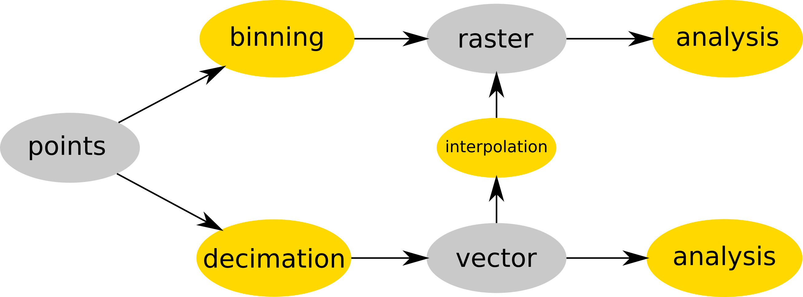
Point cloud is either binned into a raster (e.g. r.in.lidar) and then analyzed as raster or optionally decimated (e.g. using v.in.lidar), converted to vector (still using v.in.lidar) and then interpolated (e.g. v.surf.rst) into raster or analyzed as a vector (e.g. v.vect.stats). Data are in gray, processes in yellow.
-
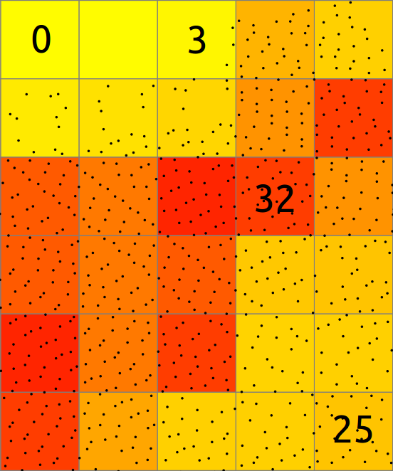
In basic case, binning of points into a 2D raster consists of counting the number of points falling into each cell. The resulting cell value is then count of points in that cell.
-
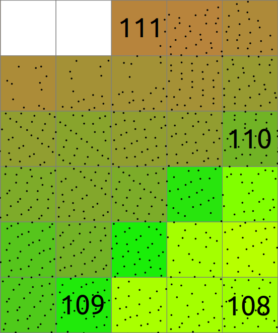
In general binning involves also values associated with the points and computes statistics on these values. Here the mean of Z coordinates of all the point in each cell is computed and stored in the raster. The cells without any points are NULL (NoData) shown in white here.


Fastest way to analyze basic properties of a point cloud is to use binning and create a raster map. We will now use r.in.lidar to create point count (point density) raster. At this point, we don't know the spatial extent of the point cloud, so we cannot set computation region ahead, but we can tell the r.in.lidar module to determine the extent first and use it for the output using the -e flag. We are using a course resolution to maximize the speed of the process.
r.in.lidar input=.../nc_tile_0793_016_spm.las output=count_10 method=n -e resolution=10
Now we can see the distribution patter, but let's examine also the numbers:
r.info map=count_10
Since there is a lot of points per one cell, we can use a finer resolution:
r.in.lidar input=.../nc_tile_0793_016_spm.las output=count_1 method=n -e resolution=1
Now we have appropriate number of points in most of the cells and there are no density artifacts around the edges, so we can use this raster as the base for extent and resolution we will use from now on.
g.region raster=density_1 -p
This region settings means a lot of cells and many of them would be empty, esp. when we start filtering the point cloud. To account for that, we can modify just the resolution of the computational region:
g.region res=3 -ap
Use binning to obtain the ground surface (ground is class 2):
r.in.lidar input=.../nc_tile_0793_016_spm.las output=ground class_filter=2
Change the color table to use the elevation colors and not the default:
r.colors map=ground color=elevation
Compute shaded relief:
r.relief input=ground output=relief
Now combine the shaded relief raster and the elevation raster. This can be done in several ways. In GUI by changing opacity of one of them. A better result can be obtained using the r.shade module which combines the two rasters and creates a new one. Finally, this can be done on the fly without creating any raster using the d.shade module. The module can be used from GUI through toolbar or using the Console tab:
d.shade shade=relief color=ground
So far we used number of points in a cell to compute density and mean elevation of points in a cell to determine the ground surface. Now we will use binning again but with computing range of elevation (Z) values of points:
r.in.lidar input=.../nc_tile_0793_016_spm.las output=range method=range
To understand what the map shows, compute statistics using r.report:
r.report map=tile_range_6m units=c
This shows that there is an outlier (at around 600 m). Change the color table to histogram equalized to see the contrast in the rest of the map:
r.colors map=tile_range_6m color=viridis -e
Now when we know the outlier and the expected range of values, use the zrange parameter to filter out any possible outliers. Since the raster map called range already exists, use the overwrite flag, i.e. --overwrite in the command line or checkbox in the GUI.
r.in.lidar input=.../nc_tile_0793_016_spm.las output=range method=range zrange=0,200 --overwrite
Interpolation
Now we will interpolate a digital surface model (DSM) and for that we can increase resolution to obtain as much detail as possible (use 0.5 m for high detail or 2 m for speed):
g.region -pa res=0.5
Before interpolating, let's confirm that the spatial distribution of the points allows us to safely interpolate. We need to use the same filters as we will use for the DSM itself:
r.in.lidar input=.../nc_tile_0793_016_spm.las output=count_interpolation method=n return_filter=first zrange=0,300
First we import LAS file as vector points, we keep only first return points and limit the import vertically to avoid using outliers found in the previous step. If using GUI, uncheck add to before running it.
v.in.lidar -obt input=.../nc_tile_0793_016_spm.las output=first_returns return_filter=first zrange=0,300
Then we interpolate:
v.surf.rst input=tile_points elevation=tile_dsm tension=25 smooth=1 npmin=100
Now we could visualize the resulting DSM by computing shaded relief with r.relief or by using 3D view (see the following sections).
Terrain analysis
Set the computational region based on an existing raster map:
g.region raster=density_1
Check if the point density is sufficient:
r.in.lidar input=.../nc_tile_0793_016_spm.las output=count_ground method=n class_filter=2 zrange=0,300
Import points:
v.in.lidar -obt input=.../nc_tile_0793_016_spm.las output=points_ground class_filter=2 zrange=0,300
The interpolation will take some time, but we can set the computational region to a smaller area to save some time before we determine what are the best parameters for interpolation. This can be done in the GUI from the Map Display toolbar or here just quickly using the prepared coordinates:
g.region n=223751 s=223418 w=639542 e=639899
Now we interpolate the ground surface using regularized spline with tension (implemented in v.surf.rst) and at the same time we also derive slope, aspect and curvatures (the following code is one long line):
v.surf.rst input=points_ground tension=25 smooth=1 npmin=100 elevation=terrain slope=slope aspect=aspect pcurvature=profile_curvature tcurvature=tangential_curvature mcurvatur=mean_curvature
When we examine the results, especially the curvatures curvatures show a pattern which may be caused by some problems with the point cloud collection. We decrease the tension which will cause the surface to hold less to the points and we increase the smoothing. We just replace the existing raster by the new one using the --overwrite flag shortened to --o.
v.surf.rst input=points_ground tension=20 smooth=5 npmin=100 elevation=terrain slope=slope aspect=aspect pcurvature=profile_curvature tcurvature=tangential_curvature mcurvatur=mean_curvature --o
When we are satisfied with the result, we get back to our desired raster extent:
g.region raster=density_1
And finally interpolate the ground surface in the full extent:
v.surf.rst input=points_ground tension=20 smooth=5 npmin=100 elevation=terrain slope=slope aspect=aspect pcurvature=profile_curvature tcurvature=tangential_curvature mcurvatur=mean_curvature --o
Instead of using r.relief, we will use r.skyview:
r.skyview input=terrain output=skyview ndir=8 colorized_output=terrain_skyview
Combine the terrain and skyview also on the fly:
d.shade shade=skyview color=terrain
Analytical visualization based on shaded relief:
r.shaded.pca input=terrain output=pca_shade
Local relief model:
r.local.relief input=terrain output=lrm shaded_output=shaded_lrm
Pit density:
r.terrain.texture elevation=terrain thres=0 pitdensity=pit_density
Finally, we use automatic detection of landforms (using 50 m search window):
r.geomorphon -m elevation=terrain forms=landforms search=50
Vegetation analysis

zrange parameter filters out points which don't fall into the specified range of Z valuesCoarser resolution is more appropriate for vegetation as we need to pull more points together for the statistics (3 m):
g.region raster=density_1 res=3
We use all the points, but with the Z filter to get the range of heights in each cell:
r.in.lidar input=.../nc_tile_0793_016_spm.las output=range method=range zrange=0,200
Or lower res to avoid gaps (and possible smoothing during their filling).
r.in.lidar -d input=.../nc_tile_0793_016_spm.las output=height_above_ground method=max base_raster=terrain
In case we if(height_above_ground > 2, height_above_ground, null()).
r.mapcalc "height_above_2m = if(height_above_ground > 2, 1, null())"
Use r.grow to extend the patches and fill in the holes:
r.grow input=height_above_2m output=vegetation
We consider the result to represent the vegetated areas. We clump (connect) the individual cells into patches using r.clump):
r.clump input=vegetation output=veg_clump
r.area input=vegetation_clump output=veg_size lesser=100
r.to.vect -s input=vegetation_size output=vegetation type=area
g.region res=1
r.in.lidar -e -i input=.../nc_tile_0793_016_spm.las output=intensity zrange=0,300
r.fill.gaps --overwrite input=intensity output=intensity_filled uncertainty=uncertainty distance=3 mode=wmean power=2.0 cells=8
r.colors map=intensity_filled color=grey
r.colors -e map=intensity_filled color=grey
r3.in.lidar -d input=.../nc_tile_0793_016_spm.las n=count sum=intensity_sum mean=intensity proportional_n=prop_count proportional_sum=prop_intensity base_raster=terrain
r3.to.rast input=prop_count output=slices_prop_count
r3.colors
Second Map Display and Animation Tool
Bonus tasks
3D visualization

We can explore our study area in 3D view (use image on the right if clarification is needed for below steps):
- Add raster dsm and uncheck or remove any other layers. Any layer in Layer Manager is interpreted as surface in 3D view.
- Switch to 3D view (in the right corner of Map Display).
- Adjust the view (perspective, height).
- In Data tab, set Fine mode resolution to 1 and set ortho as the color of the surface (the orthophoto is draped over the DSM).
- Go back to View tab and explore the different view directions using the green puck.
- Go again to Data tab and change color to viewshed raster computed in the previous steps.
- Go to Appearance tab and change the light conditions (lower the light height, change directions).
- When finished, switch back to 2D view.
Classify ground and non-ground points
v.lidar.mcc input=points_all ground=mcc_ground nonground=mcc_nonground
Optimizations, troubleshooting and limitations
Speed optimizations:
- rasterize early (often less cells than points, natural spatial index, many algorithms use it)
- if you can rasterize, decimate
- binning is much faster than interpolation
- faster count-based decimation performs the same on a given point cloud for terrain as slower grid-based decimation (Petras et al. 2016)
- r.in.lidar
- choose computation region extent and resolution ahead
- have enough memory to avoid using percent option (high memory usage versus high I/O)
- v.in.lidar
- -r limit import to computation region extent
- -t do not create attribute table
- -b do not build topology (applicable to other modules as well)
- -c store only coordinates, no categories or IDs
Memory requirements:
- r.in.lidar
- depend on the side of output and type of analysis
- can be reduced by percent option
- ERROR: G_malloc: unable to allocate ... bytes of memory
- on Linux available memory for process is RAM + SWAP partition
- v.in.lidar
- low when not building topology
- for topology and low memory use export GRASS_VECTOR_LOWMEM=1 (os.environ['GRASS_VECTOR_LOWMEM'] = '1' in Python)
Limits:
- vector features with topology: count limit is about 2 billion features per vector map 2^31 - 1
- points without topology: count theoretically limited only by the 64bit architecture (may be 16 exbibytes per file but depends on the file system)
- for large vectors with attributes PostgreSQL backend is recommended
- more limits for 32bit versions for operations which require memory
- read/write to disk often limits speed (faster for rasters in 7.1)
- number of open files limitation (system limit)
- often 1024, change using ulimit on Linux
- r.watershed 90,000 x 100,000 (9 billion cells) in 77.2 hours (2.93GHz)
- v.surf.rst: minutes = 1.5e-11 * points^2 (test: 13 min for 1 million points and 201880 cells)
- Read the documentation.
- Write to grass-user mailing list or GRASS GIS bug tracker in case you hit limits. For example, if you get negative number as the number of points or cells, open a ticket.
Bleeding edge
Processing point clouds as 3D rasters
r3.forestfrag r3.count.categories r3.scatterplot
Point profiles
v.profile.points
PDAL integration
v.in.pdal, r.in.pdal, ... use PDAL as backend for import and export – v.in.pdal, v.in.points, or v.in.lidar provide access to selected PDAL analyses – v.pdal or in one of v.in.pdal, v.in.points, v.in.lidar
r.in.kinect
Has some features from r.in.lidar, v.in.lidar, and PCL (Point Cloud Library), but the point cloud is continuously updated from a Kinect scanner using OpenKinect libfreenect2 (used in Tangible Landscape).
d.points
show large point clouds in Map Display (2D) – d.points
Store return and class information as category
general support for color stored as category
See also
- GRASS GIS at FOSS4G Boston 2017
- From GRASS GIS novice to power user (workshop at FOSS4G Boston 2017)
- Analytical data visualizations at ICC 2017
- Unleash the power of GRASS GIS at US-IALE 2017
- Creating animation from FUTURES output in GRASS GIS
- Introduction to GRASS GIS with terrain analysis examples
- Lidar Analysis of Vegetation Structure
- LIDAR
- GRASS GIS and Python
- GRASS GIS and R
- GRASS Location Wizard
External links and references:
- Petras, V., Newcomb, D. J., Mitasova, H. 2017. Generalized 3D fragmentation index derived from lidar point clouds. In: Open Geospatial Data, Software and Standards. DOI:10.1186/s40965-017-0021-8
- Petras, V., Petrasova, A., Jeziorska, J., Mitasova, H. 2016. Processing UAV and lidar point clouds in GRASS GIS. ISPRS - International Archives of the Photogrammetry, Remote Sensing and Spatial Information Sciences XLI-B7, 945–952, 2016 (full text at ResearchGate)
- Processing lidar and general point cloud data in GRASS GIS (slides)
- Petrasova, A., Mitasova, H., Petras, V., Jeziorska, J. 2017. Fusion of high-resolution DEMs for water flow modeling. In: Open Geospatial Data, Software and Standards. DOI: 10.1186/s40965-017-0019-2