Lidar Analysis of Vegetation Structure

This exercise was initially created as a session in a GIS training for the U. S. Fish and Wildlife Service in May, 2016 by Doug Newcomb.

Session Objectives

At the conclusion of this session, you will be able to:

• Open GRASS GIS and Create a Location from an existing file
• Link external raster elevation data to the Location
• Import LAS point cloud data to assess DEM accuracy
• Import LAS point cloud data to create various vegetation structure products
• Export raster vegetation structure data layers from GRASS to GeoTiff

Material Created By: Doug Newcomb (May 2016)

Software: GRASS 7.2

Directory Path: D:\grasslidar (assumed at some places, use any directory you want)

Image Files: D05_37_20026801_20141209.tif D05_37_20026803_20141209.tif D05_37_20026802_20141209.tif D05_37_20026804_20141209.tif

LAZ format LiDAR files: LA_37_20026801_20141209.laz LA_37_20026803_20141209.laz LA_37_20026802_20141209.laz LA_37_20026804_20141209.laz

Data can be accessed online here

Elevation data is commonly used in landscape analysis, but it is also quite useful in vegetation analysis. This exercise will walk you through basic analysis of a LiDAR point cloud to better understand vegetation structure.

All data are located in c:\grasslidar\data, unless otherwise noted.

Step 1: Creating GRASS Workspace

The first thing to do when starting to work in GRASS is to create a Location. GRASS Locations are single projection areas with a defined resolution and extent. The initial location can be easily created from an existing data set.

In Windows, Click on Start-->All Programs-->GRASS GIS 7.2--> GRASS GIS 7.2 GUI

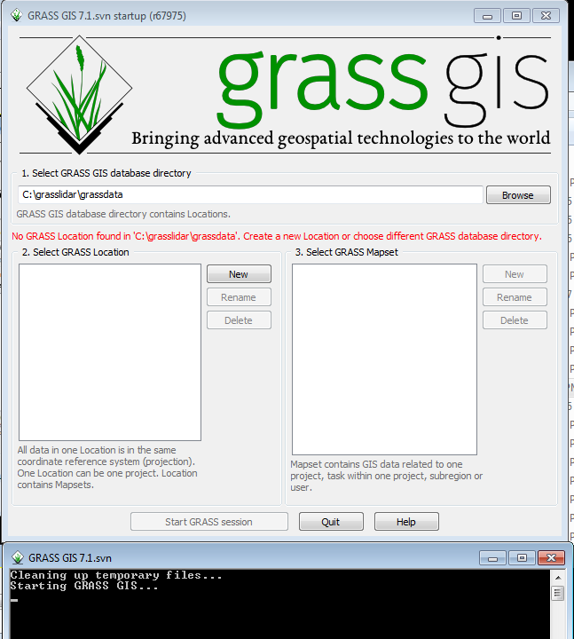
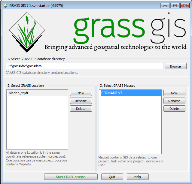
Two windows will open, the GRASS startup window ( to select or create a workspace) and the GRASS command prompt.

• Click on the New button between the Location and Mapset windows. This will bring up the menu to define a new Location.

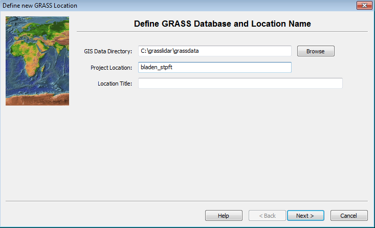
The GIS Data Directory is where all of your grass workspaces will reside. Creating a new directory with a unique name for grass data is recommended. This directory can be created anywhere that the user has write access. Project location is a subdirctory name for this particular project. Like with ArcGIS, it is best to avoid spaces in Directory names to avoid problems down the road. Click on the Browse button and select c:\grasslidar\grassdata. The data is from Bladen County, NC and is in the North Carolina State Plane NAD83(2011) projection with units feet, so call it bladen_stpft

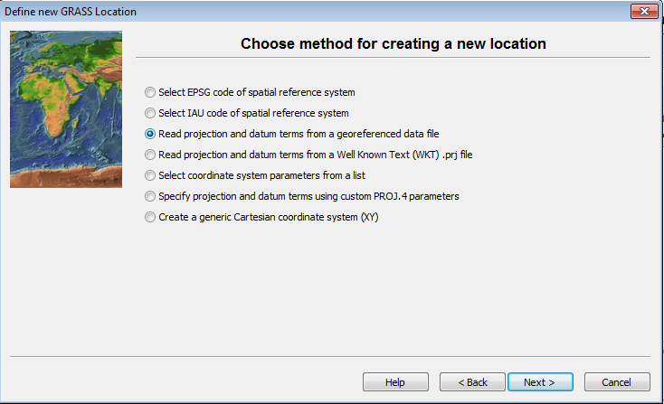
• Enter the Data Directory and Project Location – this brings up the location creation method menu

• Click on the radio button for Read projection and datum terms from a georeferenced file.
• Click Next

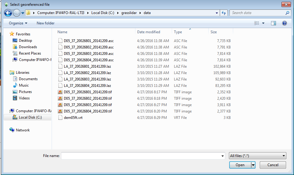
This brings up the georeferenced file dialog.

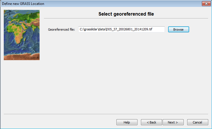
• Browse to C:\grasslidar\data and look at the data available:

In this directory, you will see 4 file types: asc, laz, tif, and vrt. LiDAR data is usually distributed as tiles of point clouds and Digital Elevation Models (DEMs) ASC and TIFF are common file formats to distribute DEM data. Asc is an ArcInfo ASCII Grid file, which is simply a text file representing a grid and does not have any projection data associated with it. Generally .tif files distributed as DEMs have projection information embedded in the file. LAZ is an open method of compression for LAS files. VRT is a virtual raster index of the 4 .tif files in this directory.

In this directory, and select D05_37_20026801_20141209.tif as the georeferenced file. 

• Click Next.

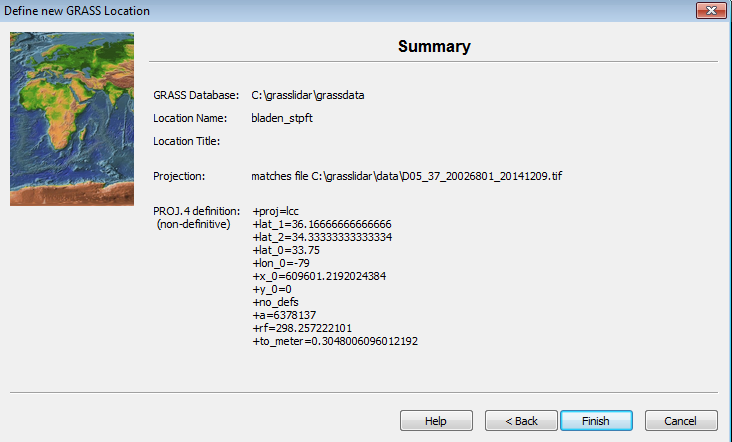
GRASS reads the georeference data from the elevation file and displays the projection data.

• Click Finish

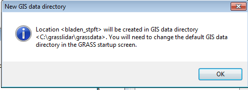
The next message relates to setting a default path for GRASS startup.

• Click OK

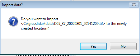
In the following message, you have the option if importing the data set you used for georeferencing the workspace.

• Click No

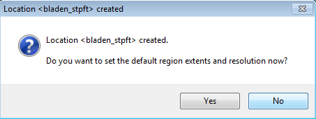
The location has been created. You are prompted to set the default region extents and resolution.

• Click No

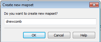
You are then prompted to create a new mapset.

• Click Cancel

You have finished creating a Location with the default PERMANENT mapset. The next time GRASS is started, you can either select an existing Location and Mapset, create a new Mapset within the Location, or create a new Location.

• Click on the PERMANENT Mapset
• Click Start GRASS session

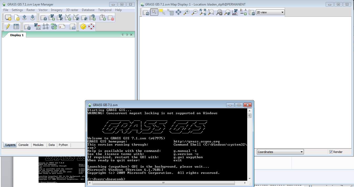
You will then see the Layer Manager Window, the Map Display Window for Display 1.

Step 2: Adding a data layer

We are now ready to add data to the Mapset. We can either import Raster and Vector data using the GDAL translation library, or we can link to existing external data sets read only to reduce data duplication. In this case, we will link to the 1m elevation data we used to create the Location using the r.external command.

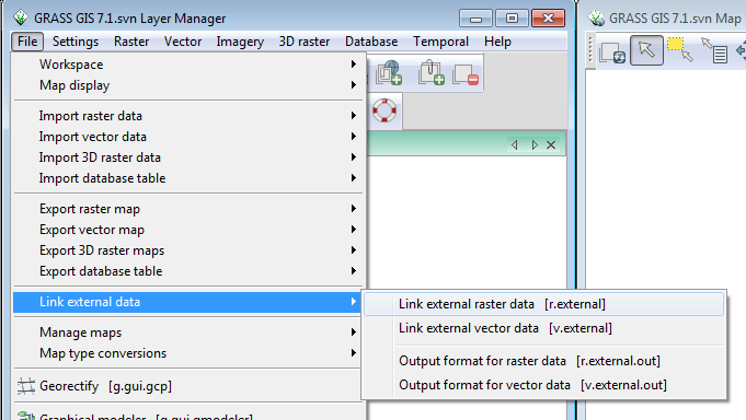
• In the Layer Manager window, click File-->Link external data-->Link external raster data.

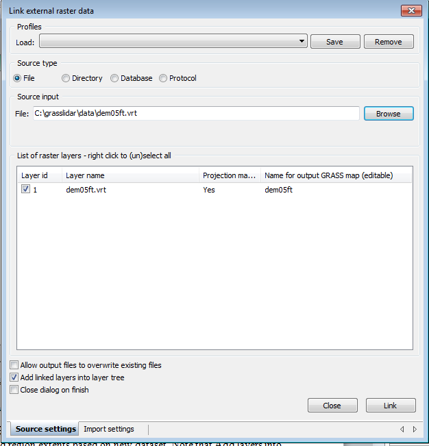
This brings up the r.external dialog.

We would like to treat the 4 tiles of LiDAR and elevation data as a single seamless unit, to accomplish this, we are going to first select the demo05ft.vrt image index as our input raster.

• Browse to C:\grasslidar\data\dem05ft.vrt and select it. Note that the Add layers into layer tree is checked. For large data sets, leave this unchecked.
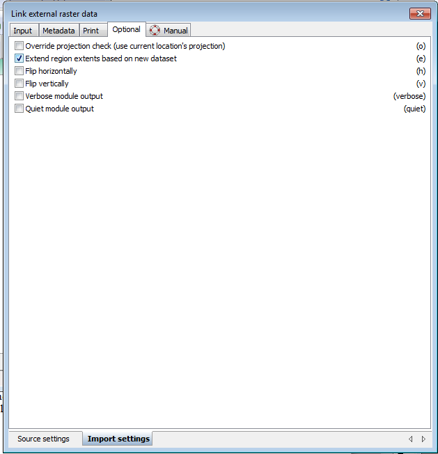
• Click on the import settings tab at the bottom
• Click on the box for Extend region extents based on new dataset.

• Click back to the Source settings tab and Click Link.

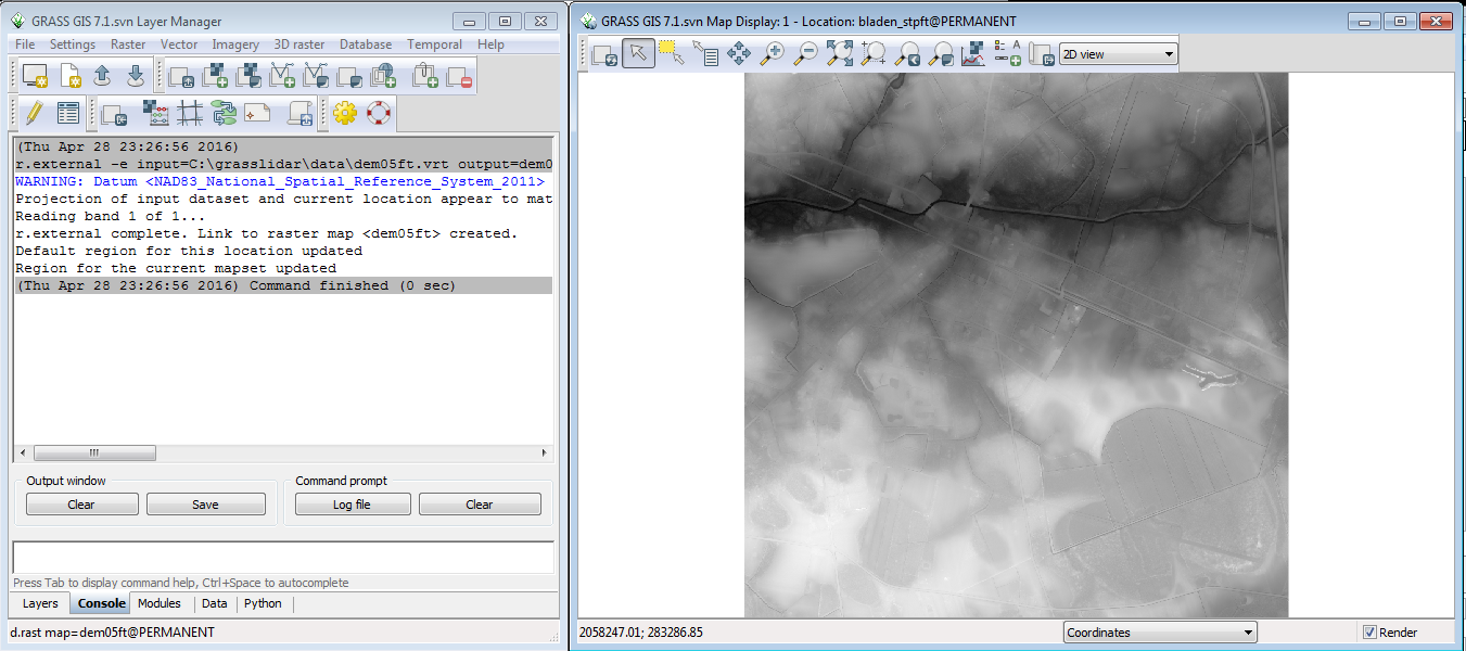
The Layer Manager window will switch to the Command console tab and display the results of the r.external command . Click the close button on the r.external dialog.

The 4 DEM rasters are displayed in the Map Display window as a single seamless data set . Any GIS software built with Geodata Abstraction Library(GDAL) ( including ArcGIS 10.0 and above) will see a vrt mosaic as a single raster layer. Creating the vrt is as simple as going to the black GRASS command window ,navigating to the directory in the with the rasters and typing: gdalbuildvrt dem05ft.vrt *.tif

For larger data sets, it takes much less time to link to a raster data set than import it and linking also saves on storage space.

Step 3: Setting up the region

The region in a GRASS mapset defines the extent and resolution of the results of any raster actions. To make sure that all of a raster layer is affected by a command, it is customary to set the region’s extent and resolution to match the raster layer. To set the region to match the elevation raster that we just linked to ,

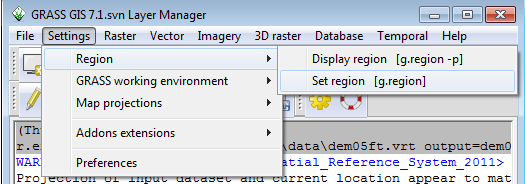
• From the Layer Manager window drop down options, click the Settings-->Region-->Set region

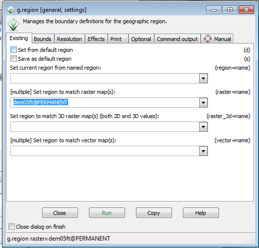
• In the g.region menu, in the Set region to match raster map section, use the drop down to select dem05ft@Permanent.
• Click Run

When the command finishes, your will see “Command finished” and the time taken in the g.region window .

• Click Close in the g.region window
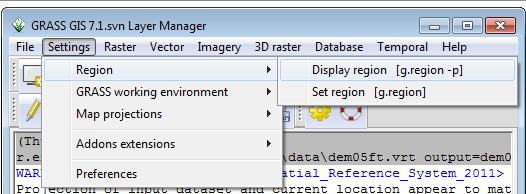
• Click Settings-->Region-->Display region

In the command console tab of the Layer Manager window, you see the current region definintion: resolution, bounds, rows and columns. The output resolution of raster layers created will usually match the region resolution. To change the output resolution, you will need to change the resolution of the region.

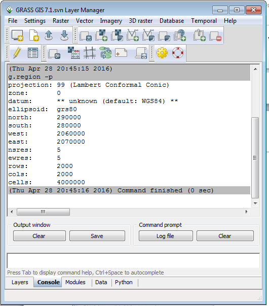
A quick note about the results. The datum is not recognised and assumed to be WGS84 by GRASS. The datum is NAD83 (2011). The data coordinates have not changed, the datum information has not been recognized on import. We can work with the data and assign the correct datum information after export from GRASS. This should be corrected by the final release of this version of GRASS.

Step 4: Processing the Lidar data

There are 4 lidar tiles that correspond to the 4 tiles of elevation data. The data is in the Compressed LAS files (laz) format. LASZip, http://www.laszip.org/, is an open compression method that losslessly compresses LAS format LiDAR data files to about 25 -30 percent of the original size.

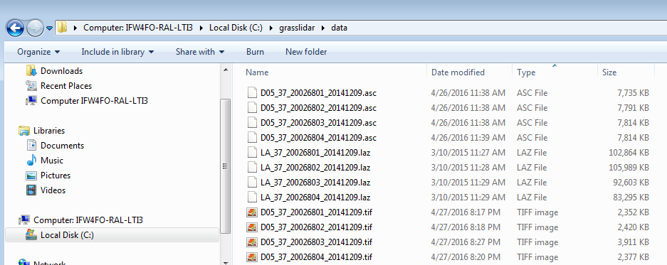
You will be using the GRASS 7.1 r.in lidar. R.in.lidar uses a binning process, performing an analysis on the points that fall in each raster cell. It’s best to process las tiles as a single unit to avoid border effects. There are two ways to do this: 1) Merge the las files together into a single file using tools such as lastools lasmerge, https://rapidlasso.com/lastools/lasmerge/ . Many software packages are still limited to LAS format 1.2 which can only handle up to 4.2 billion points per file ( a current limitation in GRASS7.1) . This option can also take up hard drive space. 2) The second option available in r.in.lidar is to give a filename with a list of adjacent LAS/LAZ files and it will treat it as a virtual seamless LiDAR data set. If you look in the data directory, you will see laslist.txt. The contents of the file are: C:\grasslidar\data\LA_37_20026801_20141209.laz C:\grasslidar\data\LA_37_20026802_20141209.laz C:\grasslidar\data\LA_37_20026803_20141209.laz C:\grasslidar\data\LA_37_20026804_20141209.laz

This is a list of the compressed las files in the directory that you will be processing. Give r.in.lidar c:\grasslidar\data\laslist.txt as the input file list, and it will treat all 4 files as a single point cloud. This method has been tested on file lists up to 966 las files.

This exercise will use the second method. To start r.in.lidar, go to File-->Import raster data-->LAS Lidar points import.

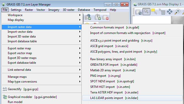
This will bring up the r.in.lidar menu.

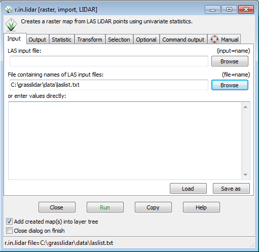
You will notice that there are several tabs across the top of the command window. The first tab is the Input tab . You can either enter the name of the individual las or laz file, or you can enter the name of a txt file with a list of las or laz files. In the second option, browse to the location of the laslist.txt file and select it as shown.

Next we will set the output raster layer.

• Click on the Output tab
• In the Name for output raster layer box, type “ bladen_test_5ft_pt_count” as the output layer