Lidar Analysis of Vegetation Structure: Difference between revisions
⚠️Dnewcomb (talk | contribs) (More of the exercise) |
⚠️Dnewcomb (talk | contribs) (Add geomorphon section) |
||
| Line 403: | Line 403: | ||
[[File:Grasslidar_49.png| Geomorphon Classes]]<br /> | [[File:Grasslidar_49.png| Geomorphon Classes]]<br /> | ||
For this activity, we will use the simple 10 class calculation. Outputs will be cells with the following classes: Flat, peak, ridge, shoulder, spur, slope hollow, footslope, valley, and pit. | |||
To do our terrain classification, we will need to load the r.geomorphon addon to GRASS. | |||
GRASS has an online repository of Addons much like QGIS has for plugins. Most addons do not require administrative access to install. | |||
* In the Layer Manager window, click on Settings-->Addons extentions-->Install extention from addons | |||
[[File:Grasslidar_50.png| Addon Menu]]<br /> | |||
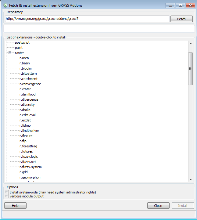
This will open the Fetch and install extension window. GRASS commands are named by their function: r.* commands are raster commands, v.* commands are vector commands, i.* commands are image analysis commands. | |||
* Click on the + next to raster to expand the view on all raster commands | |||
[[File:Grasslidar_51.png| Addon Selection]]<br /> | |||
* Select r.geomorphon | |||
* Click install | |||
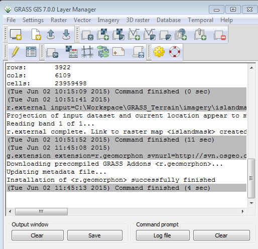
In the Layer Manager window you can follow the progress of the installation. | |||
[[File:Grasslidar_52.png| Addon Installation]]<br /> | |||
In this case, downloading and installing the addon took 4 seconds on a 2010 vintage Windows 7 laptop. | |||
== Step 6: Running r.geomorphon == | |||
The r.geomorphon command documentation is at http://grass.osgeo.org/grass70/manuals/addons/r.geomorphon.html and the publications for the technique can be found at the end of the command description. | |||
To start r.geomorphon, | |||
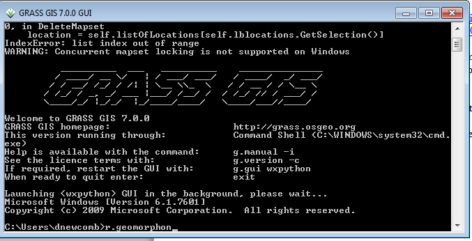
In the GRASS Command window, type r.geomorphon and press Enter. | |||
[[File:Grasslidar_53.png| Start r.geomorphon]]<br /> | |||
Entering the command without arguments brings up the r.geomorphon menu. You will notice that there are tabs across the top. The first tab is the Required Tab, with required data inputs to run the command. | |||
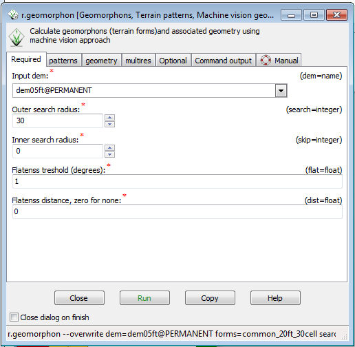
* From the dropdown for Input DEM, dem05ft@PERMANENT ( remember, the current resolution for the region is 20ft. GRASS will take the center value of the 5ft DEM in each 20ft cell and use that for the 20ft cell value, your output raster will be 20ft resolution) | |||
* In the Outer search radius, enter 30 ( number of cells around each cell to analyze) This is a very flat area, so the number may need to be higher to extract some features. | |||
[[File:Grasslidar_54.png| R.geomorphon setup]]<br /> | |||
You will note that as the command arguments are entered, they are echoed across the bottom. | |||
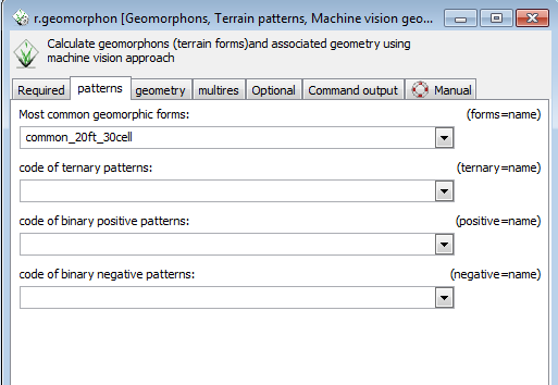
* Click on the patterns tab. | |||
* Type common_20ft_30cell in the box under Most common geomorphic forms. | |||
[[File:Grasslidar_55.png| R.geomorphon setup 2]]<br /> | |||
* Click Run | |||
The tab will immediately switch to the Command Output tab, the command options will be echoed , and a progress bar will show the progress of the command. | |||
You will need to manually add the result to the Display. | |||
* At the top of the Layer Manager window, Click Add raster map layer button | |||
Revision as of 03:15, 8 November 2016
This exercise was initially created as a session in a GIS training for the U. S. Fish and Wildlife Service in May, 2016 by Doug Newcomb.
Session Objectives
At the conclusion of this session, you will be able to:
- Open GRASS GIS and Create a Location from an existing file
- Link external raster elevation data to the Location
- Import LAS point cloud data to assess DEM accuracy
- Import LAS point cloud data to create various vegetation structure products
- Export raster vegetation structure data layers from GRASS to GeoTiff
Material Created By: Doug Newcomb (May 2016)
Software: GRASS 7.2
Directory Path: D:\grasslidar (assumed at some places, use any directory you want)
Image Files: D05_37_20026801_20141209.tif D05_37_20026803_20141209.tif D05_37_20026802_20141209.tif D05_37_20026804_20141209.tif
LAZ format LiDAR files: LA_37_20026801_20141209.laz LA_37_20026803_20141209.laz LA_37_20026802_20141209.laz LA_37_20026804_20141209.laz
Data can be accessed online here
Elevation data is commonly used in landscape analysis, but it is also quite useful in vegetation analysis. This exercise will walk you through basic analysis of a LiDAR point cloud to better understand vegetation structure.
All data are located in c:\grasslidar\data, unless otherwise noted.
Step 1: Creating GRASS Workspace
The first thing to do when starting to work in GRASS is to create a Location. GRASS Locations are single projection areas with a defined resolution and extent. The initial location can be easily created from an existing data set.
In Windows, Click on Start-->All Programs-->GRASS GIS 7.2--> GRASS GIS 7.2 GUI
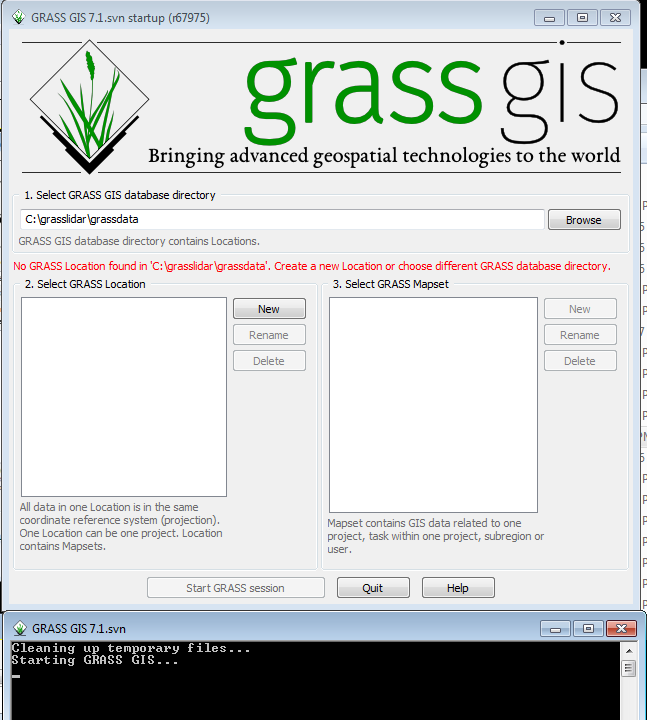
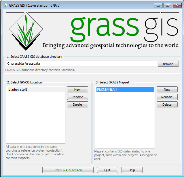
Two windows will open, the GRASS startup window ( to select or create a workspace) and the GRASS command prompt.
- Click on the New button between the Location and Mapset windows. This will bring up the menu to define a new Location.
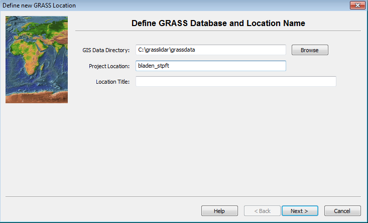
The GIS Data Directory is where all of your grass workspaces will reside. Creating a new directory with a unique name for grass data is recommended. This directory can be created anywhere that the user has write access. Project location is a subdirctory name for this particular project. Like with ArcGIS, it is best to avoid spaces in Directory names to avoid problems down the road. Click on the Browse button and select c:\grasslidar\grassdata. The data is from Bladen County, NC and is in the North Carolina State Plane NAD83(2011) projection with units feet, so call it bladen_stpft
- Enter the Data Directory and Project Location – this brings up the location creation method menu
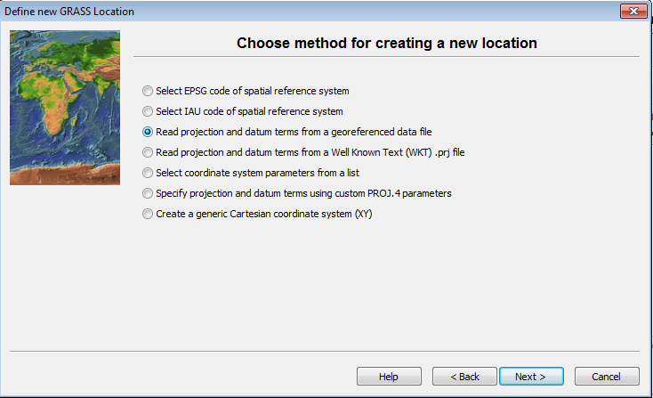
- Click on the radio button for Read projection and datum terms from a georeferenced file.
- Click Next
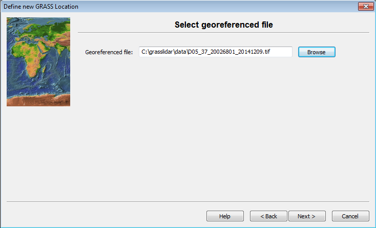
This brings up the georeferenced file dialog.
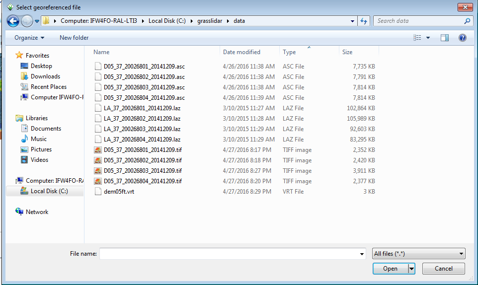
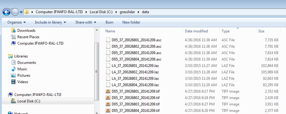
- Browse to C:\grasslidar\data and look at the data available:
In this directory, you will see 4 file types: asc, laz, tif, and vrt. LiDAR data is usually distributed as tiles of point clouds and Digital Elevation Models (DEMs) ASC and TIFF are common file formats to distribute DEM data. Asc is an ArcInfo ASCII Grid file, which is simply a text file representing a grid and does not have any projection data associated with it. Generally .tif files distributed as DEMs have projection information embedded in the file. LAZ is an open method of compression for LAS files. VRT is a virtual raster index of the 4 .tif files in this directory.
In this directory, and select D05_37_20026801_20141209.tif as the georeferenced file.
- Click Next.
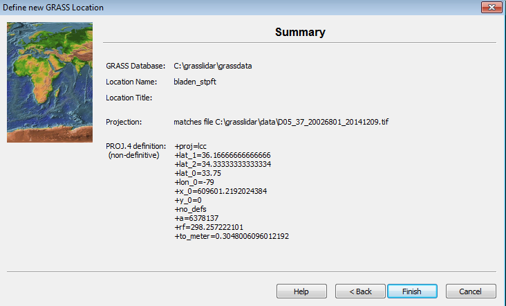
GRASS reads the georeference data from the elevation file and displays the projection data.
- Click Finish
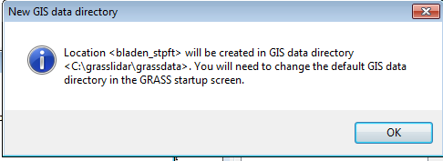
The next message relates to setting a default path for GRASS startup.
- Click OK
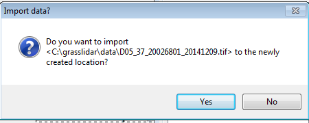
In the following message, you have the option if importing the data set you used for georeferencing the workspace.
- Click No
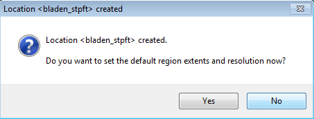
The location has been created. You are prompted to set the default region extents and resolution.
- Click No
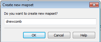
You are then prompted to create a new mapset.
- Click Cancel
You have finished creating a Location with the default PERMANENT mapset. The next time GRASS is started, you can either select an existing Location and Mapset, create a new Mapset within the Location, or create a new Location.
- Click on the PERMANENT Mapset
- Click Start GRASS session
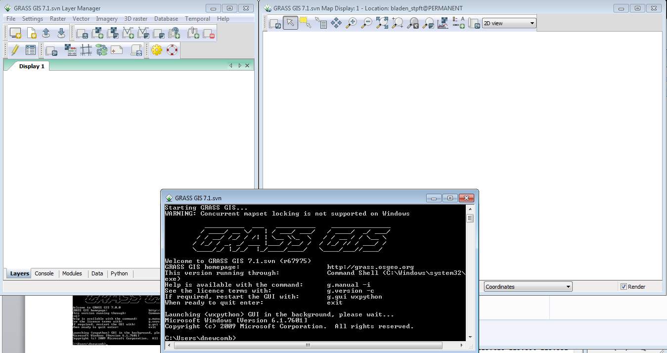
You will then see the Layer Manager Window, the Map Display Window for Display 1.
Step 2: Adding a data layer
We are now ready to add data to the Mapset. We can either import Raster and Vector data using the GDAL translation library, or we can link to existing external data sets read only to reduce data duplication. In this case, we will link to the 1m elevation data we used to create the Location using the r.external command.
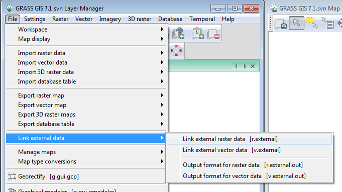
- In the Layer Manager window, click File-->Link external data-->Link external raster data.
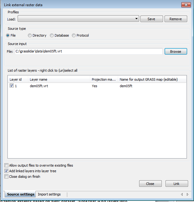
This brings up the r.external dialog.
We would like to treat the 4 tiles of LiDAR and elevation data as a single seamless unit, to accomplish this, we are going to first select the demo05ft.vrt image index as our input raster.
- Browse to C:\grasslidar\data\dem05ft.vrt and select it. Note that the Add layers into layer tree is checked. For large data sets, leave this unchecked.
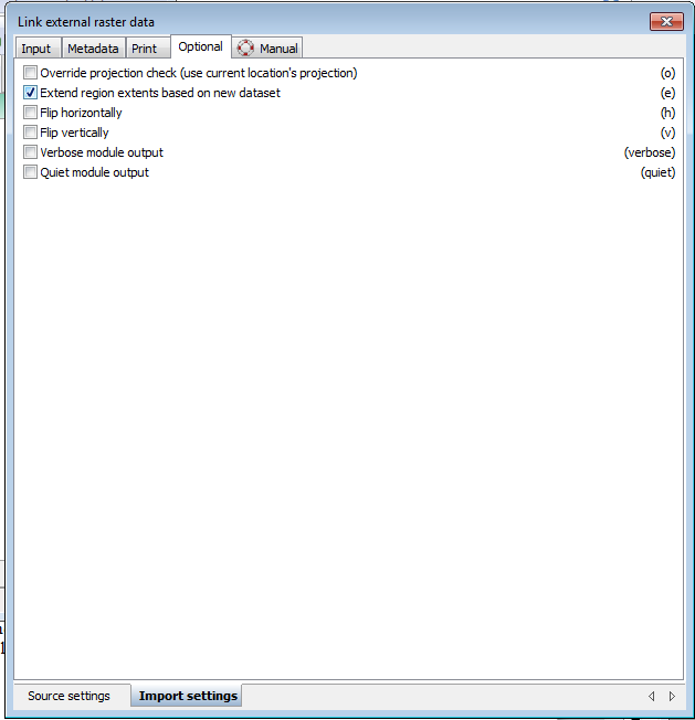
- Click on the import settings tab at the bottom
- Click on the box for Extend region extents based on new dataset.
- Click back to the Source settings tab and Click Link.
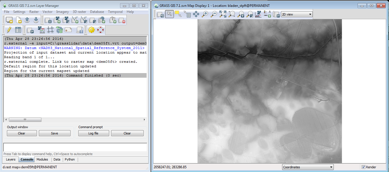
The Layer Manager window will switch to the Command console tab and display the results of the r.external command . Click the close button on the r.external dialog.
The 4 DEM rasters are displayed in the Map Display window as a single seamless data set . Any GIS software built with Geodata Abstraction Library(GDAL) ( including ArcGIS 10.0 and above) will see a vrt mosaic as a single raster layer. Creating the vrt is as simple as going to the black GRASS command window ,navigating to the directory in the with the rasters and typing: gdalbuildvrt dem05ft.vrt *.tif
For larger data sets, it takes much less time to link to a raster data set than import it and linking also saves on storage space.
Step 3: Setting up the region
The region in a GRASS mapset defines the extent and resolution of the results of any raster actions. To make sure that all of a raster layer is affected by a command, it is customary to set the region’s extent and resolution to match the raster layer. To set the region to match the elevation raster that we just linked to ,
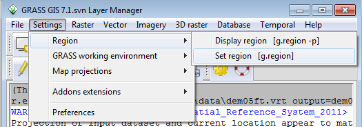
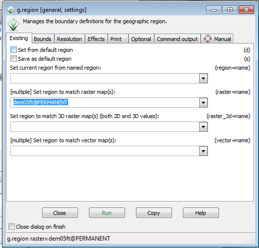
- From the Layer Manager window drop down options, click the Settings-->Region-->Set region
- In the g.region menu, in the Set region to match raster map section, use the drop down to select dem05ft@Permanent.
- Click Run
When the command finishes, your will see “Command finished” and the time taken in the g.region window .
- Click Close in the g.region window
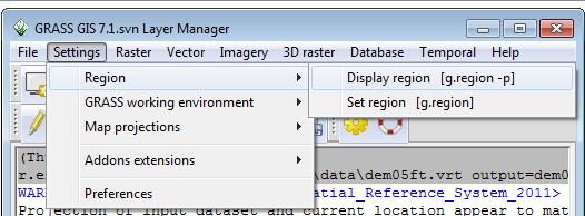
- Click Settings-->Region-->Display region
In the command console tab of the Layer Manager window, you see the current region definintion: resolution, bounds, rows and columns. The output resolution of raster layers created will usually match the region resolution. To change the output resolution, you will need to change the resolution of the region.
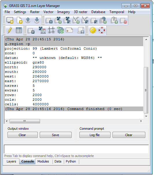
A quick note about the results. The datum is not recognised and assumed to be WGS84 by GRASS. The datum is NAD83 (2011). The data coordinates have not changed, the datum information has not been recognized on import. We can work with the data and assign the correct datum information after export from GRASS. This should be corrected by the final release of this version of GRASS.
Step 4: Processing the Lidar data
There are 4 lidar tiles that correspond to the 4 tiles of elevation data. The data is in the Compressed LAS files (laz) format. LASZip, http://www.laszip.org/, is an open compression method that losslessly compresses LAS format LiDAR data files to about 25 -30 percent of the original size.
You will be using the GRASS 7.1 r.in lidar. R.in.lidar uses a binning process, performing an analysis on the points that fall in each raster cell. It’s best to process las tiles as a single unit to avoid border effects. There are two ways to do this: 1) Merge the las files together into a single file using tools such as lastools lasmerge, https://rapidlasso.com/lastools/lasmerge/ . Many software packages are still limited to LAS format 1.2 which can only handle up to 4.2 billion points per file ( a current limitation in GRASS7.1) . This option can also take up hard drive space. 2) The second option available in r.in.lidar is to give a filename with a list of adjacent LAS/LAZ files and it will treat it as a virtual seamless LiDAR data set. If you look in the data directory, you will see laslist.txt. The contents of the file are: C:\grasslidar\data\LA_37_20026801_20141209.laz C:\grasslidar\data\LA_37_20026802_20141209.laz C:\grasslidar\data\LA_37_20026803_20141209.laz C:\grasslidar\data\LA_37_20026804_20141209.laz
This is a list of the compressed las files in the directory that you will be processing. Give r.in.lidar c:\grasslidar\data\laslist.txt as the input file list, and it will treat all 4 files as a single point cloud. This method has been tested on file lists up to 966 las files.
This exercise will use the second method. To start r.in.lidar, go to File-->Import raster data-->LAS Lidar points import.
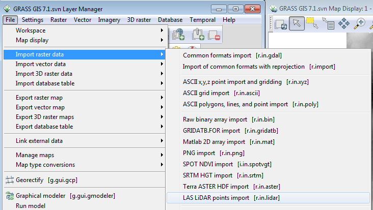
This will bring up the r.in.lidar menu.
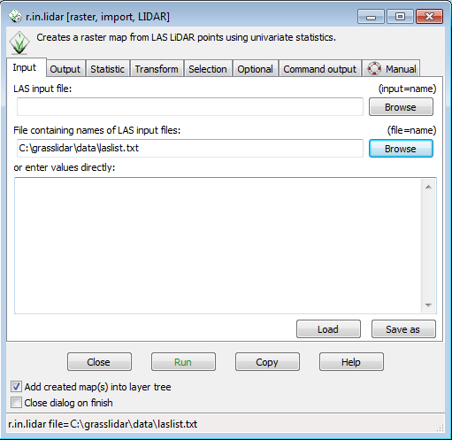
You will notice that there are several tabs across the top of the command window. The first tab is the Input tab . You can either enter the name of the individual las or laz file, or you can enter the name of a txt file with a list of las or laz files. In the second option, browse to the location of the laslist.txt file and select it as shown.
Next we will set the output raster layer.
- Click on the Output tab
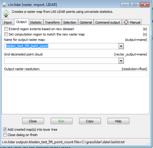
- In the Name for output raster layer box, type “ bladen_test_5ft_pt_count” as the output layer
You will be binning the data using a 5ft resolution cell. In this case, you will be counting how many LiDAR returns are in each 5ft cell.
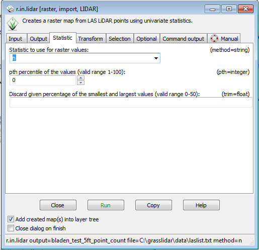
- Click on the Statistic tab
- Select n from the Statistic to use for raster values drop down menu
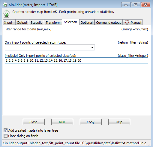
- Click on the selection tab
- You want all points except the low noise ( class 7) so put 1,2,3,4,5,6,8,9,10,11,12,13,14,15,16,17,18,19,20 into the box for “Only import points of selected classes.” (feel free to copy and paste)
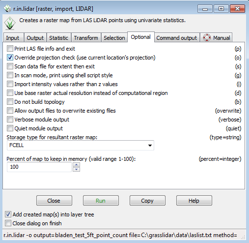
- Click on the Optional tab
- Select the check box for Override projection check
- Click Run.
Your display should look like this, with the result of the point count automatically added to the display.
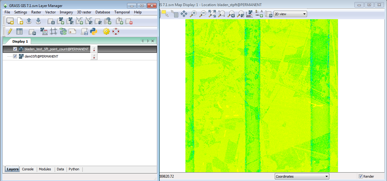
To add a legend to the display:
- Click on the Add map elements button on the top of the Display window
- Select show/hide legend
The default legend is not clear for this data set, so simplify the legend by:
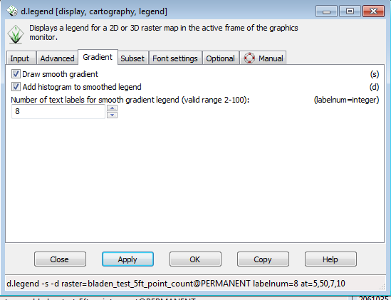
- Double clicking on the legend to bring up the d.legend menu.
- Click on the Gradient tab and check the Draw smooth gradient and Add histogram to smoothed legend.
- Change the number of text labels from the default of 5 to 8.
- Click OK
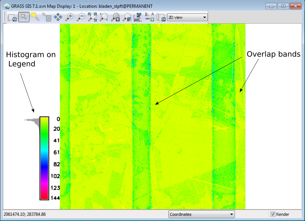
As you can see in the illustration above, the histogram on the legend tells you that most of the cells have fewer than 10 points per cell. For any valid statistical analysis of the point values in the cell you would need to pick a cell size larger than 5ft if you are performing statistics on the point values within each cell.
You can also see the overlap of the LiDAR data collection flight lines. This makes the use of direct point count density useless as a measure of vegetation density unless all overlap points are removed.
Step 6: Canopy Heights and Other Forest Structure Metrics
Calculation of canopy heights involves determining the distance between the ground and the top of the vegetation. It can be done two steps , creating a digital surface model (DSM) and subtracting the Digital Elevation Model (DEM) With GRASS, this can be done in one step.
Go back to the r.in.lidar menu:
- Set the output raster to bladen_test_5ft_ch.
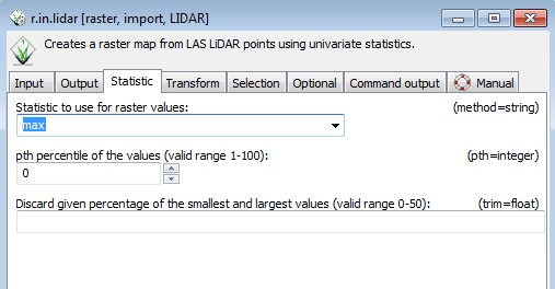
- Go to the statistic tab and select max from the drop down menu.
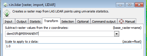
- Select the Transform tab
- From the Subtract raster values from the z coordinates, select dem05ft from the dropdown menu.
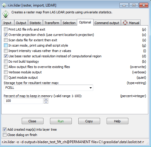
- Go to the Optional tab
- Check the boxes next to Override projection check and Use base raster actual resolution instead of computational region
- Click Run
- Select the Display window and double-click on the legend.
- Select as the input raster layer bladen_test_05ft_ch
You have just used the 5 ft resolution DEM to convert the z values of the point cloud to height above ground. Selecting the maximum value in each cell now gives the canopy height in each cell. Using this proceedure allows you to convert the LiDAR point Z values to height above ground at the 5ft resolution, but the calculations after the conversion will be done for the cell size of the current resolution of the location.
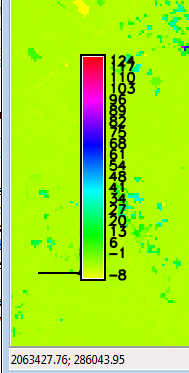
Look back at the legend. You will notice that the bottom value is negative 4. Why is that? Run r.in.lidar again with the statistic st to min and the output raster set to bladen_test_05ft_min.
- Go back to d.legend and set the raster to bladen_test_05ft_min.
- Click on the Gradient tab and set the number of text labels to 20
- Click apply
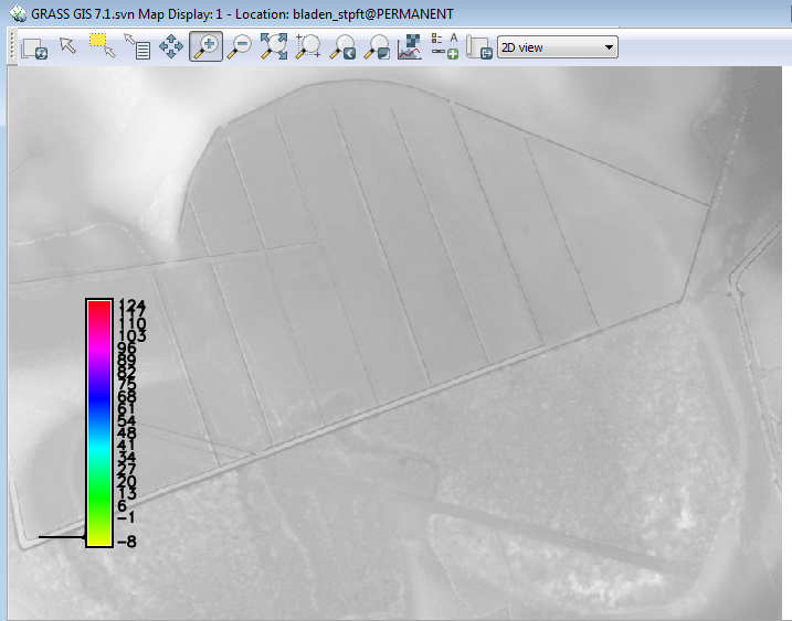
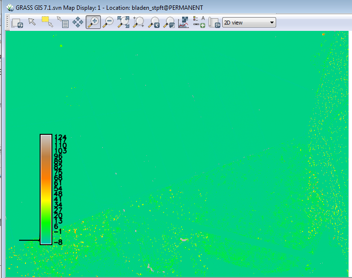
You can see that the bulk of the minimum values are less than the DEM surface. Turn off all layers except the DEM layer. Zoom into the large oval area in the Southeast corner of the DEM.
This feature is called a Carolina bay. The northern half has been ditched and drained, and the southern half remains in the native thick vegetation. Turn the min values back on.
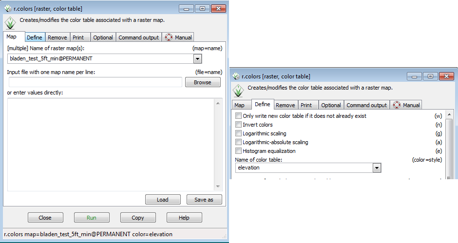
- Go to raster-->Manage colors --> Color tables. This will open the r.colors menu.
- Select the Define tab and in the Name of color table dropdown select elevation.
You will notice that in the light green and yellowish areas are significantly above the DEM surface. This is an indication that the laser did not penetrate the vegetation to hit the ground. While the DEM is not perfect, it gives us a better ground surface than just using the min value. There are ways to work around those differences, but that is not the topic for today.
Look at the other end
- Set the region to match the 5ft dem
- Remove the base raster in the Transform tab and in the Optional tab
- Remove the zrange on the Selection tab
- Set the output raster to top_of_canopy_5ft
- Run r.in.lidar with the max method
Change your legend to match the top of canopy layer. What is the max height that you see?
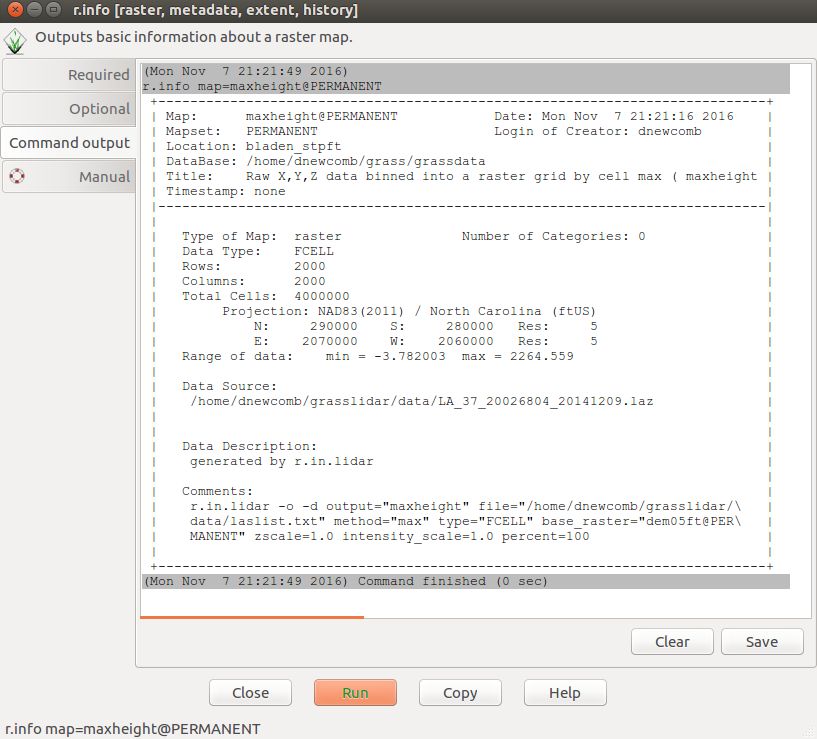
- Click Raster-->Reports and statistics-->Basic raster metadata (r.info)
- Select dem05ft
- Click Run
R.info gives basic information about the raster layer. You see the rows, columns, number of cells, projection, the command that created the raster is listed as well. This is all useful information for metadata construction. The min and max values of the raster is what you need to look at now. The maximum value in the DEM is 2264.559. Since we have no trees in NC over 200ft, it seems we have some invalid high points. To remedy this:*
- Go back to the Selection tab and and
- for the zrange enter -10,250.
- Click Run
This gives a -10, 250 range around the high and low ground in the area (93-10 =83 and 128+250 = 378). This should exclude most of the extraneous points and leave a 5 ft resolution Digital Surface Model(DSM). Change the legend to display the new raster layer. What differences do you see?
For now we are going to leave this dataset, but we will come back to it later.
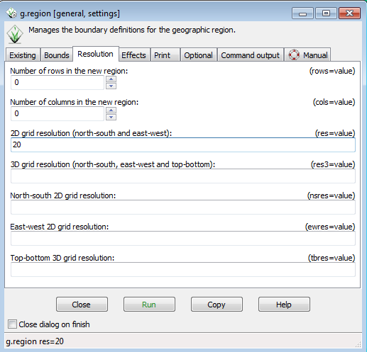
- Go back to Settings-->Region--> Set region to open the g.region dialog.
- Select the Resolution tab.
- Enter 20 in the 2D grid resolution box
- Click Run
If you go to Settings-->Region-->Display region You will see : nsres: 20 ewres: 20
The Region resolution setting is now for 20ft cells.
- Go back to the r.in.lidar menu and:
- Set the output raster to bladen_test_20ft_ch and
- Set the statistic to max.
- Set the transform layer back to dem05ft
- Check the box for use base raster resolution
- Click Run
- Set the legend to bladen_test_20ft_ch
The Z values were converted to height above ground using the 5ft DEM and then statistics were calculated for 20ft cells. Notice how you see the outlines of the ditches.
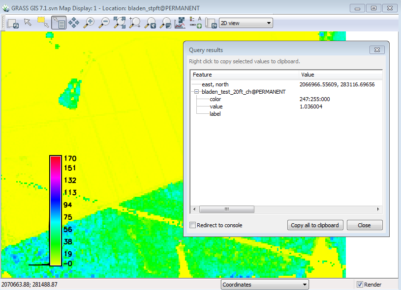
- Make sure that the bladen_test_20ft_ch is highlighted
- Click on the Query selected raster/vector button ( 4th from the left in the display window)
- Place the crosshairs on one of the ditches
- Left Click
A window will pop up giving the location coordinates, the layer being queried, the color of the feature, and the value of the feature. In this case, the canopy height of the feature. The Z conversion to height above ground is not perfect and may depend on the accuracy of the DEM and the steepness of the slope represented by the raster.
Remember that a slope is a smooth surface that is being interpolated to a grid format.
Choosing a cell size can be important. At a 20ft resolution, you will be getting parts of larger trees and 60ft may be more appropriate to capture a more completepicture of the landscape vegetaion. Converting to height above ground allows for the use of cells of arbitrary size. Your analysis can match up with the cell size and footprint to exactly match the cell alignment of existing data.
There are several other statistical measures that are available in r.in lidar: n, mean, range, sum, standard deviation, variance, coefficeint of variance, median,percentile, skewness, trimmean. Mean height, variance and skewness are metrics used in vegetation analysis.
At the 20ft resolution, repeat r.in.lidar for variance and mean methods. What differences do you see in the resulting rasters?
Repeat r.in.lidar at 20ft resolution using n as the statistic to create a point count layer.
- Go to the Selection tab and
- Set the z range to 3,10
- Set the output raster to bladen_20ft_shrub_count
- Click Run
- Go to the Selection tab
- Set the zrange to 10,20
- Set the output raster to bladen_20ft_midstory_count
- Click Run
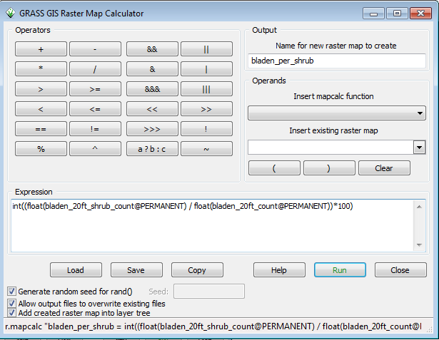
As stated above, using the raw point count is not suitable for vegetation analysis in areas where there are overlaps in collection. However, if horizontal sections of the point counts per cell are divided by the total point count per cell you can compare the percentage of the points that occur in horizontal sections. In this case, we will be using raster algebra to divide the shrub and midstory point counts by the total point counts using r.mapcalc, https://grass.osgeo.org/grass71/manuals/r.mapcalc.html .
- Go to Raster-->Raster map calculator (r.mapcalc)
This will open the r.mapcalc menu:
- Enter bladen_per_shrub in the Name for new raster map to create
- Use the dropdown in the Insert existing raster map section to select bladen_20ft_shrub_count
- Click on the / button for division
- Use the dropdown to select bladen_20ft_count
Now things get interesting. The point count rasters are integers. Mathmatical operations between integers results in an integer. Dividing an integer by a larger integer number results in a number less than one. In an integer grid, this truncates to 0.
To get around this, you convert each integer grid before the operation to a floating point grid, so bladen_20ft_shrub becomes float(bladen_20ft_shrub) and bladen_20ft_count becomes float(bladen_20ft_count) and you divide one floating point grid by another floating point grid and you get a floating point grid.
Multiply this floating point grid by 100 to put the values back in the range of 100 to 0. Finally, convert results of the entire operation back to an integer grid by enclosing it with int() . The final command in the Expression box is:
int((float(bladen_20ft_shrub_count@PERMANENT)/float(bladen_20ft_count@PERMANENT))*100)
The resulting raster should look like this:
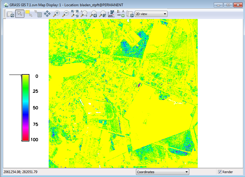
Repeat the exercise with the midstory layer and compare the two layers. Do you see differences between the shrub and midstory percentage of points layers?
We will continue the vegetation analysis, but first we need to take a short side trip into terrain analysis that will relate back to our vegetation analysis.. Terrain analysis will be done using geomrphons.
Step 5: Terrain analysis with geomorphons
What are geomorphons? Geomorphon is a new technique for classifying terrain based on a line of sight analysis, see http://geomorphometry.org/system/files/StepinskiJasiewicz2011geomorphometry.pdf
and , http://www.sciencedirect.com/science/article/pii/S0169555X12005028
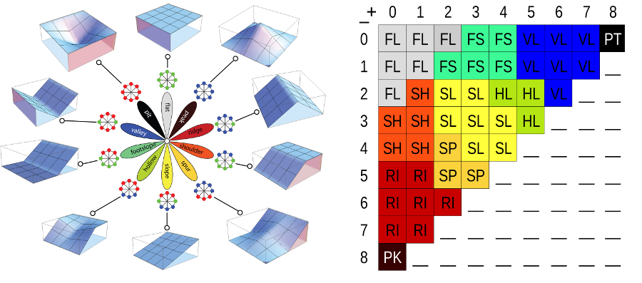
The technique uses a line of sight metric for terrain form calculation. There are options for a simple 10 class representation, a 498 class numeric coding, or positive and negative encoding per cell on line of sight.
For this activity, we will use the simple 10 class calculation. Outputs will be cells with the following classes: Flat, peak, ridge, shoulder, spur, slope hollow, footslope, valley, and pit.
To do our terrain classification, we will need to load the r.geomorphon addon to GRASS.
GRASS has an online repository of Addons much like QGIS has for plugins. Most addons do not require administrative access to install.
- In the Layer Manager window, click on Settings-->Addons extentions-->Install extention from addons
This will open the Fetch and install extension window. GRASS commands are named by their function: r.* commands are raster commands, v.* commands are vector commands, i.* commands are image analysis commands.
- Click on the + next to raster to expand the view on all raster commands
- Select r.geomorphon
- Click install
In the Layer Manager window you can follow the progress of the installation.
In this case, downloading and installing the addon took 4 seconds on a 2010 vintage Windows 7 laptop.
Step 6: Running r.geomorphon
The r.geomorphon command documentation is at http://grass.osgeo.org/grass70/manuals/addons/r.geomorphon.html and the publications for the technique can be found at the end of the command description.
To start r.geomorphon,
In the GRASS Command window, type r.geomorphon and press Enter.
Entering the command without arguments brings up the r.geomorphon menu. You will notice that there are tabs across the top. The first tab is the Required Tab, with required data inputs to run the command.
- From the dropdown for Input DEM, dem05ft@PERMANENT ( remember, the current resolution for the region is 20ft. GRASS will take the center value of the 5ft DEM in each 20ft cell and use that for the 20ft cell value, your output raster will be 20ft resolution)
- In the Outer search radius, enter 30 ( number of cells around each cell to analyze) This is a very flat area, so the number may need to be higher to extract some features.
You will note that as the command arguments are entered, they are echoed across the bottom.
- Click on the patterns tab.
- Type common_20ft_30cell in the box under Most common geomorphic forms.
- Click Run
The tab will immediately switch to the Command Output tab, the command options will be echoed , and a progress bar will show the progress of the command. You will need to manually add the result to the Display.
- At the top of the Layer Manager window, Click Add raster map layer button
