R.basin
Introduction
The module r.basin has been designed to perform the delineation and the morphometric characterization of a given basin, on the basis of an elevation raster map and the coordinates of the outlet. Please note that it is designed to work only in projected coordinates. Here a tutorial based on NC sample dataset is presented. The tutorial refers to GRASS 6. In GRASS 7, a few improvements have been introduced to r.basin. See the section below for details.
Preparation
As a first step, we set the computational region to match the elevation raster map:
g.region rast=elevation@PERMANENT -ap
projection: 99 (Lambert Conformal Conic)
zone:       0
datum:      nad83
ellipsoid:  a=6378137 es=0.006694380022900787
north:      228500
south:      215000
west:       630000
east:       645000
nsres:      10
ewres:      10
rows:       1350
cols:       1500
cells:      2025000
For the basin's delineation, a pair of coordinates is required. Usually coordinates belonging to the natural river network don't exactly match with the calculated stream network. What we should do is to calculate the stream network first, and then to find the coordinates on the calculated stream network closest to the coordinates belonging to the natural stream network.
# Calculate flow accumulation map (MFD)
r.watershed -af elevation=elevation@PERMANENT accumulation=accum

# Extract the stream network
r.stream.extract elevation=elevation@PERMANENT accumulation=accum threshold=20 stream_rast=stream_network stream_vect=streams
We no longer need the accumulation map:
g.remove rast=accum
Now that we have the calculated stream network, we should choose a pair of coordinates for the outlet belonging to it. Let's choose for example:
easting=636654.791181 northing=218824.126649
We no longer need the stream network map:
g.remove rast=stream_network
Preparation for multiple basins' analysis
If there are a lot of basins to be analysed, the coordinate pairs of the intersections between the calculated stream network and basins (outlet points) can be found by:
# Convert basins polygon vector boundaries to lines
v.type input=basinspoly output=basinsline type=boundary,line

# Patch basins lines with stream network
v.patch input=basinsline,streams output=basins_streams

# Find cross points at intersections
v.clean input=basins_streams output=basins_streams_clean error=crosspoints_err tool=break

# Add categories to cross points vector
v.category input=crosspoints_err output=crosspoints

# Add table to cross points vector with columns for category, x and y coordinates
v.db.addtable map=crosspoints columns="cat integer,xcoor double precision, ycoor double precision"

# Upload category to cross points attribute table
v.to.db map=crosspoints option=cat columns=cat

# Upload x and y coordinates to cross points attribute table
v.to.db map=crosspoints option=coor columns=xcoor,ycoor
At this point we can create a text file called crosspoints with the coordinates in this form:
xcoor1 ycoor1
xcoor2 ycoor2
xcoor3 ycoor3
...
Now we can parse this coordinates file in order to create a new file called commands in which we'll have the r.basin commands for each sub-watershed, ready to be run in a GRASS session. Let's create a script in python for parsing:
#!/usr/bin/env python

# Open the ''crosspoints'' text file to read the coordinates
fin = open("crosspoints","r")

# Create the ''commands'' text file
fout = open("commands","w")

# Read the ''crosspoints'' lines
linesout = (line.rstrip().split() for line in fin)

# Build the r.basin command
# Put your threshold parameter instead of threshold=10000 and the name of your DEM instead of map=elevation
cmd = 'r.basin map=elevation prefix=bas%s easting=%s northing=%s threshold=10000\n'

# Write the file ''commands''
fout.writelines(cmd % (n, easting, northing) for n,(easting,northing) in enumerate(linesout))
This is a Python script, it is supposed to run externally from GRASS GIS. Save this script as parsing.py in a separate folder on your Desktop, and put the file crosspoints in such folder. To run it, open a terminal and type:
cd yourfolder
python parsing.py
Now in the same folder you will find the file commands, in which we have the r.basin commands to run in GRASS.
Usage
We can run r.basin:
r.basin map=elevation@PERMANENT prefix=out coordinates=636654.791181,218824.126649 threshold=20 dir=tmp/my_basin
Prefix parameter is a string given by the user in order to distinguish all the maps produced by every run of the program, i.e. every set of outlet's coordinates. Prefix must start with a letter.
Threshold is the same parameter given in r.watershed and r.stream.extract. Physically, it means the number of cells that determine "where the river begins". (This is an open issue for the hydrological science and a wide literature has been produced on the topic). Threshold value is usually determined by trials and errors. r.basin has a flag -a, which uses an authomatic value of threshold, corresponding to 1km^2. Such value comes from literature and is usually suitable for Italian territory, but could be definitely wrong for other territories. In order to determine the threshold, see also r.threshold and r.stream.preview.
The output of r.basin consists of:
- Several morphometric parameters, which are printed in terminal and also stored in a csv file called out_elevation_parameters.csv, in the working directory;
- Maps;
- Plots.
Morphometric parameters
The main parameters are:
- The coordinates of the vertices of the rectangle containing the basin.
- The center of gravity of the basin: the coordinates of the pixel nearest to the center of gravity of the geometric figure resulting from the projection of the basin on the horizontal plane.
- The area of the basin: is the area of a single cell multiplied by the number of cells belonging to the basin.
- The perimeter: is the length of the contour of the figure resulting by the projection of the basin on the horizontal plane.
[As a side note, a paper namely "How Long Is the Coast of Britain? Statistical Self-Similarity and Fractional Dimension" points out that perimeter is affected by a fractal problem and the number is mostly meaningless taken by itself. Hence, perimeter should never be mixed with anything from another dataset or even the same data set at a different cell resolution; it is only good as a percentage comparison to its neighbors in the same dataset].
- Characteristic values of elevation: the highest and the lowest altitude, the difference between them and the mean elevation calculated as the sum of the values of the cells divided by the number of the cells.
- The mean slope, calculated averaging the slope map.
- The length of the directing vector: the length of the vector linking the outlet to basin's barycenter.
- The prevalent orientation: is the orientation of the directing vector.
- The length of main channel: is the length of the longest succession of segments that connect a source to the outlet of the basin.
- The mean slope of main channel: it is calculated as follows:

where N is the topological diameter, i.e. the number of links in which the main channel can be divided on the basis of the junctions.
- The circularity ratio: is the ratio between the area of the basin and the area of the circle having the same perimeter of the basin.
- The elongation ratio: is the ratio between the diameter of the circle having the same area of the basin and the length of the main channel.
- The compactness coefficient: is the ratio between the perimeter of the basin and the diameter of the circle having the same area of the basin.
- The shape factor: is the ratio between the area of the basin and the square of the length of the main channel.
- The concentration time (Giandotti, 1934):

Where A is the area, L the length of the main channel and H the difference between the highest and the lowest elevation of the basin.
- The mean hillslope length: is the mean of the distances calculated along the flow direction of each point non belonging to the river network from the point in which flows into the network.
- The magnitudo: is the number of the branches of order 1 following the Strahler hierarchy.
- The max order: is the order of the basin, following the Strahler hierarchy.
- The number of streams: is the number of the branches of the river network.
- The total stream length: is the sum of the length of every branches.
- The first order stream frequency: is the ratio between the magnitudo and the area of the basin.
- The drainage density: is the ratio between the total length of the river network and the area.
- The Horton ratios (Horton, 1945; Strahler, 1957).
##################################
Morphometric parameters of basin :
##################################
Easting Centroid of basin : 635195.00
Northing Centroid of Basin : 220715.00
Rectangle containing basin N-W : 632880 , 222890
Rectangle containing basin S-E : 637010 , 218720
Area of basin [km^2] : 7.8592625
Perimeter of basin [km] : 17.7583322395
Max Elevation [m s.l.m.] : 151.7396
Min Elevation [m s.l.m.]: 94.82206
Elevation Difference [m]: 56.91754
Mean Elevation [m s.l.m.]: 127.7042
Mean Slope : 3.50
Length of Directing Vector [km] : 2.38880562659
Prevalent Orientation [degree from north, counterclockwise] :
0.913351005341
Compactness Coefficient : 5.61379074702
Circularity Ratio : 0.313175157621
Topological Diameter : 105.0
Elongation Ratio : 0.469323448397
Shape Factor : 1.16602561484
Concentration Time (Giandotti, 1934) [hr] : 3.53310944404
Length of Mainchannel [km] : 6.74021428
Mean slope of mainchannel [percent] : 1.202028
Mean hillslope length [m] : 5932.153
Magnitudo : 415.0
Max order (Strahler) : 5
Number of streams : 612
Total Stream Length [km] : 80.8272
First order stream frequency : 52.8039367562
Drainage Density [km/km^2] : 10.2843237518
Bifurcation Ratio (Horton) : 5.0940
Length Ratio (Horton) : 2.1837
Area ratio (Horton) : 5.6571
Slope ratio (Horton): 1.4418
The hypsographic curve provides the distribution of the areas at different altitudes. Each point on the hypsographic curve has on the y-axis the altitude and on the x-axis the percentage of basin surface placed above that altitude. The hypsometric curve has the same shape but is dimensionless. Quantiles of the hypsometric curve are displayed:
Tot. cells 78593.0
===========================
Hypsometric | quantiles
===========================
145 | 0.025
143 | 0.05
141 | 0.1
137 | 0.25
129 | 0.5
119 | 0.75
110 | 0.9
100 | 0.975
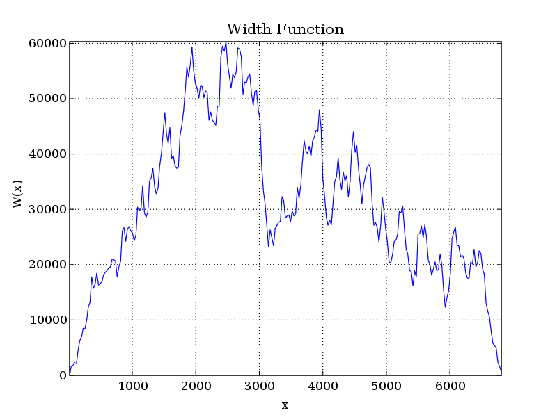
The width function W(x) gives the area of the cells in the basin at a certain flow distance x from the outlet (distance-area function). Note that the distance is not intended in the euclidean sense, but it's calculated considering the hydrological path of the water.
Tot. cells 78593.0
Tot. area 7859300.0
Max distance 6769.341392
===========================
Width Function | quantiles
===========================
801 | 0.05
1507 | 0.15
2166 | 0.3
2572 | 0.4
2958 | 0.5
3629 | 0.6
4184 | 0.7
5132 | 0.85
6089 | 0.95
The output of r.stream.stats is also displayed:
Summary:
Max order | Tot.N.str. | Tot.str.len. | Tot.area. | Dr.dens. | Str.freq.
  (num)   |    (num)   |     (km)     |   (km2)   | (km/km2) | (num/km2)
        5 |        612 |      80.8272 |    7.8593 |  10.2843 | 77.8695

Stream ratios based on regression coefficient:
 Bif.rt. | Len.rt. | Area.rt. | Slo.rt. | Grd.rt.
  5.0940 |  2.1837 |   5.6571 |  1.4418 |  1.5420

Averaged stream ratios with standard deviations:
 Bif.rt. | Len.rt. | Area.rt. | Slo.rt. | Grd.rt.
  5.5417 |  2.6271 |   5.1916 |  1.4625 |  1.6693
  3.5678 |  1.9342 |   4.3638 |  0.1448 |  0.6477

Order | Avg.len |  Avg.ar  |  Avg.sl |  Avg.grad. | Avg.el.dif
 num  |   (km)  |  (km2)   |  (m/m)  |    (m/m)   |     (m)
    1 |  0.0880 |   0.0100 |  0.0428 |     0.0331 |  3.1995
    2 |  0.2025 |   0.0501 |  0.0303 |     0.0250 |  5.3206
    3 |  0.5337 |   0.2538 |  0.0212 |     0.0177 |  8.5684
    4 |  2.7421 |   2.7104 |  0.0159 |     0.0136 | 25.1265
    5 |  1.1871 |   7.8593 |  0.0095 |     0.0051 |  6.1054

Order | Std.len |  Std.ar  |  Std.sl |  Std.grad. | Std.el.dif
 num  |   (km)  |  (km2)   |  (m/m)  |    (m/m)   |     (m)
    1 |  0.0771 |   0.0082 |  0.0362 |     0.0275 |  3.5790
    2 |  0.1841 |   0.0398 |  0.0185 |     0.0145 |  5.6062
    3 |  0.6182 |   0.2493 |  0.0131 |     0.0120 |  8.5329
    4 |  2.8546 |   3.1286 |  0.0062 |     0.0085 | 15.5228
    5 |  0.0000 |   0.0000 |  0.0000 |     0.0000 |  0.0000

Order | N.streams | Tot.len (km) | Tot.area (km2)
    1 |       490 |      43.1013 |  4.8895
    2 |        98 |      19.8470 |  4.9085
    3 |        21 |      11.2077 |  5.3290
    4 |         2 |       5.4841 |  5.4207
    5 |         1 |       1.1871 |  7.8593

Order | Bif.rt. | Len.rt. | Area.rt. | Slo.rt. | Grd.rt. | d.dens. | str.freq.
    1 |  5.0000 |  2.3024 |   0.0000 |  1.4154 |  1.3236 |  8.8151 | 100.2147
    2 |  4.6667 |  2.6353 |   5.0194 |  1.4279 |  1.4086 |  4.0434 | 19.9654
    3 | 10.5000 |  5.1378 |   5.0664 |  1.3358 |  1.3065 |  2.1031 |  3.9407
    4 |  2.0000 |  0.4329 |  10.6807 |  1.6710 |  2.6385 |  1.0117 |  0.3690
    5 |  0.0000 |  0.0000 |   2.8997 |  0.0000 |  0.0000 |  0.1510 |  0.1272
Maps
Since r.basin performs the delimitation of the river basin, all the maps produced are cropped over the basin. They are:
- Raster maps
g.list rast

out_elevation_accumulation              out_elevation_hillslope_distance
out_elevation_aspect                    out_elevation_horton
out_elevation_dist2out                  out_elevation_shreve
out_elevation_drainage                  out_elevation_slope
out_elevation_hack                      out_elevation_strahler
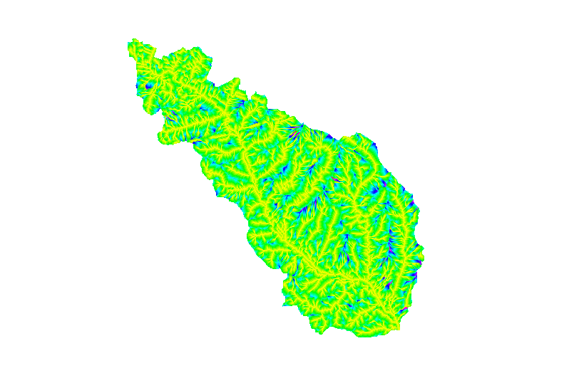
-
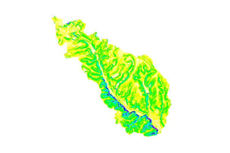
Slope
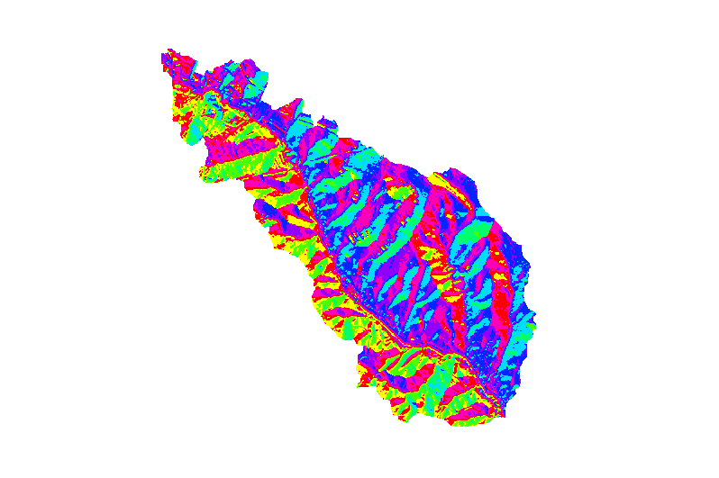
-
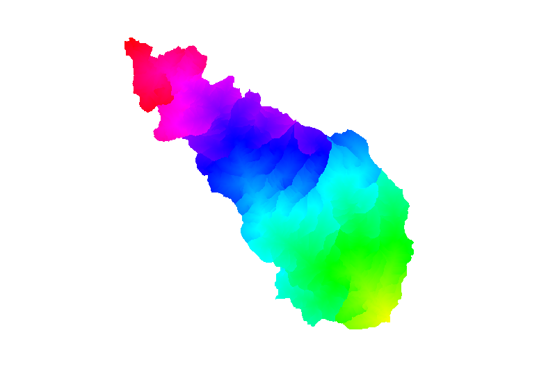
Aspect
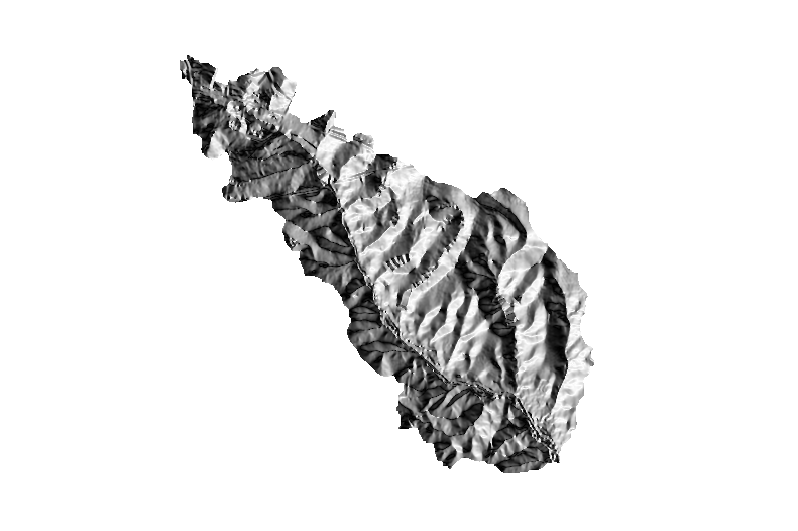
-
Flow direction
-
Flow accumulation
-
Distance to outlet (width function)
-
Length of hillslopes
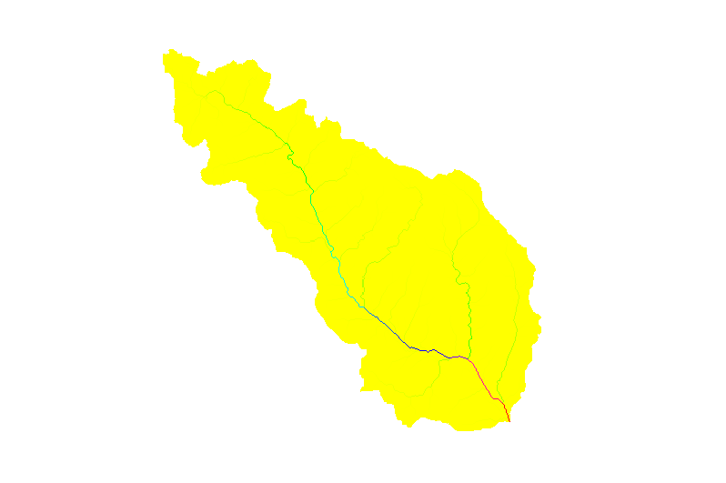
-
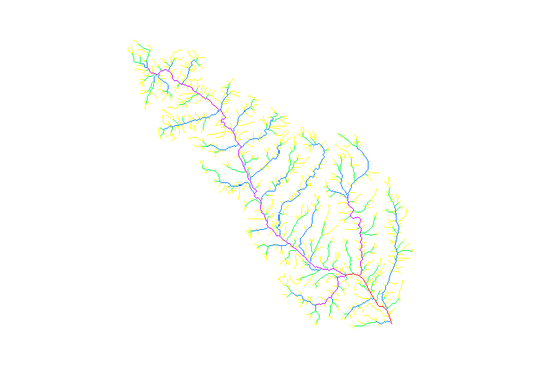
Stream network ordered according to Strahler
-
Stream network ordered according to Horton
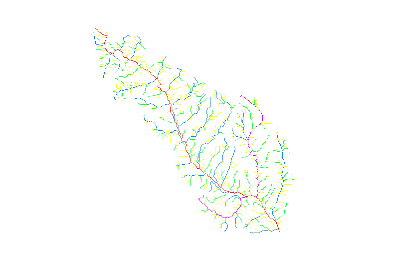
-
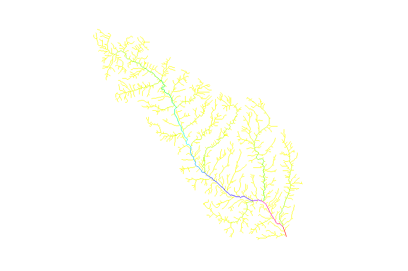
Stream network ordered according to Shreve
-
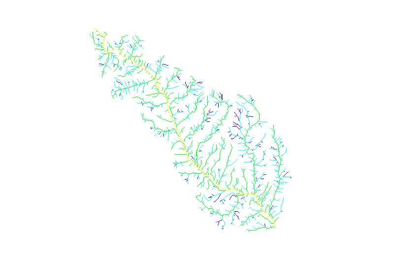
Stream network ordered according to Hack


- Vector maps
g.list vect

out_elevation_basin       out_elevation_network
out_elevation_mainchannel out_elevation_outlet
out_elevation_outlet_snap
-
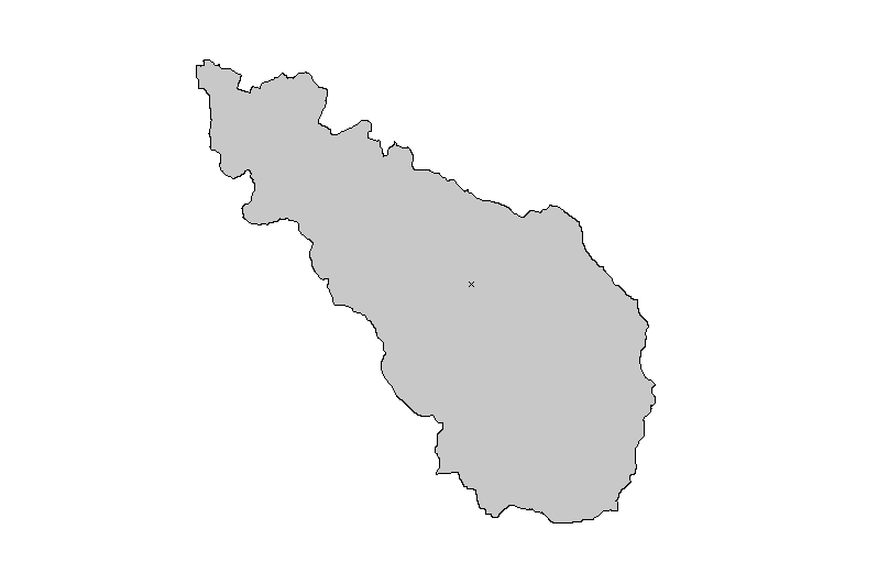
Basin
-
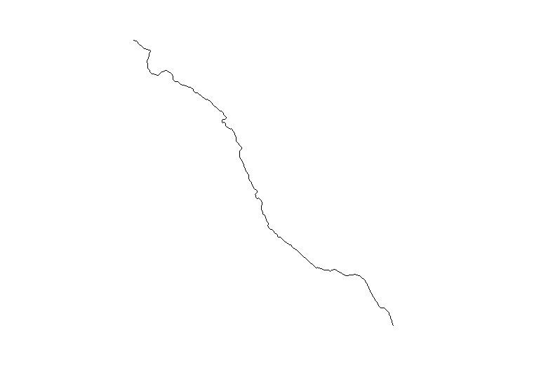
Main channel
-
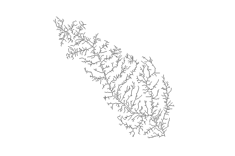
Stream network
-
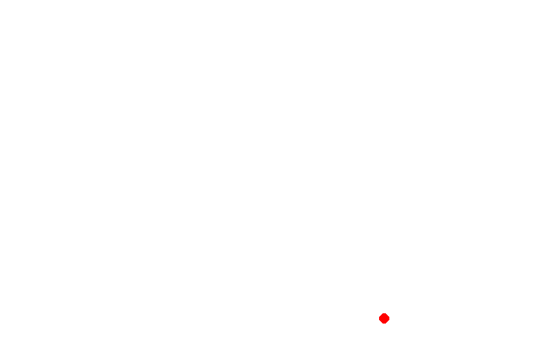
Outlet


The vector map out_elevation_outlet_snap has a table associated, that stores all the parameters calculated. The outlet_snap is the outlet moved to the nearest river network, and can slightly differ from the outlet given by the coordinates pair, in case this latter doesn't fall on the (calculated) river network.
Graphics
Graphics are stored in the working directory:
- out_elevation_ipsographic.png
- out_elevation_ipsometric.png
- out_elevation_width_function.png
-
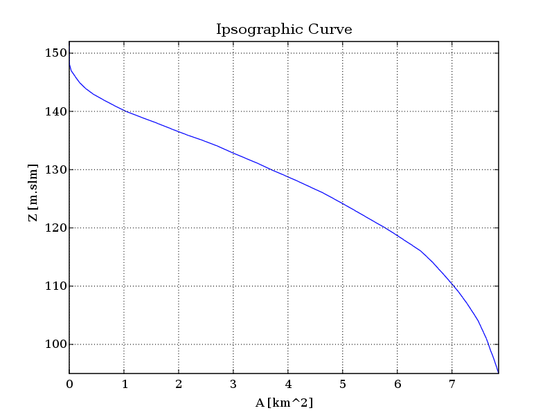
Ipsographic curve
-
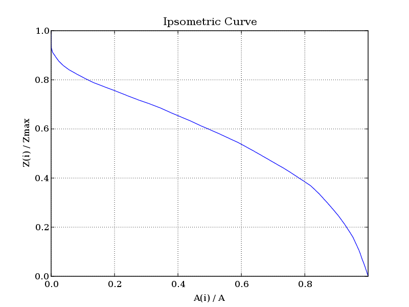
Ipsometric curve (Nondimensional ipsographic curve)
-
Width function


Known issues
- r.basin hasn't been designed for working in lat/long coordinates. This means that if you are working in lat/long coordinates, you need to reproject your map first in order to apply the tool.
- r.basin is designed to work in meters unit. The values that you get using feet are nonsense.
- r.basin does not handle overwrite. You need to delete the output products already created (maps, text file, figures) by hand before running it again.
r.basin for GRASS 6.4
r.basin was initially designed to run in grass 6.4, but in G7, r.basin has been improved and bugs were fixed, so it is strongly advised to upgrade to G7. The usage in G6 is:
r.basin [-ac] map=name prefix=prefix easting=east northing=north [threshold=threshold]
See also
References
- Di Leo Margherita, Di Stefano Massimo, An Open-Source Approach for Catchment's Physiographic Characterization, In: Proceedings of AGU Fall Meeting 2013, S.Francisco, CA, USA.
- Di Leo Margherita, Working report: Extraction of morphometric parameters from a digital elevation model - Panama. North Carolina State University, 2010 (PDF)
- Di Leo M., Di Stefano M., Claps P., Sole A., Caratterizzazione morfometrica del bacino idrografico in GRASS GIS (Morphometric characterization of the catchment in GRASS GIS environment), Geomatics Workbooks n.9, 2010. (PDF).
- Rodriguez-Iturbe I., Rinaldo A., Fractal River Basins, Chance and Self-Organization. Cambridge Press, 2001.