SOD Spread tutorial: Difference between revisions
⚠️Wenzeslaus (talk | contribs) (new URL for the dataset) |
⚠️Wenzeslaus (talk | contribs) (→Input data used in this tutorial: format of the data) |
||
| Line 15: | Line 15: | ||
* study boundaries | * study boundaries | ||
* mapset containing moisture and temperature values | * mapset containing moisture and temperature values | ||
The sample dataset is a GRASS GIS Location, so it goes into your GRASS GIS Database which is usually a directory called grassdata in your home directory or your Documents directory. | |||
= Workflow = | = Workflow = | ||
Revision as of 03:49, 8 November 2018
r.spread.sod is a model for stochastic landscape spread of the forest pathogen Sudden Oak Death. This tutorial shows how to prepare data and run the model. You can download the sample dataset and simulate sudden oak death spread in the Rouge River-Siskiyou National Forest region of western Oregon.
Software
Required software includes:
- GRASS GIS >=7.2
- Addon module:
Input data used in this tutorial
Download the sample dataset containing:
- digital elevation model
- forest density
- orthophoto of study area
- study boundaries
- mapset containing moisture and temperature values
The sample dataset is a GRASS GIS Location, so it goes into your GRASS GIS Database which is usually a directory called grassdata in your home directory or your Documents directory.
Workflow
Download sample data and unzip it. Launch GRASS GIS and select the unzipped Oregon directory, Location Oregon and create a new Mapset tutorial.
Change working directory:
Type cd (stands for change directory) into the GUI Console and hit Enter. Navigate to where ever you have saved the example data and change directory to the tutorial mapset.
Install addon:
g.extension r.spread.sod
First, we will set computational region of our analyses to an extent covering our study area and so that the cells are aligned with one of our rasters:
g.region vector=EU1_12x8 -p
Create files with lists of input maps
List all maps in the weather mapset in one text file using g.list. Search for ppt for precipitation and tmean or temperature mean for temperature:
g.list -m type=raster pattern=*ppt* mapset=weather output=precipitation.txt
g.list -m type=raster pattern=*tmean* mapset=weather output=temperature.txt
Compute the spread of SOD for default values
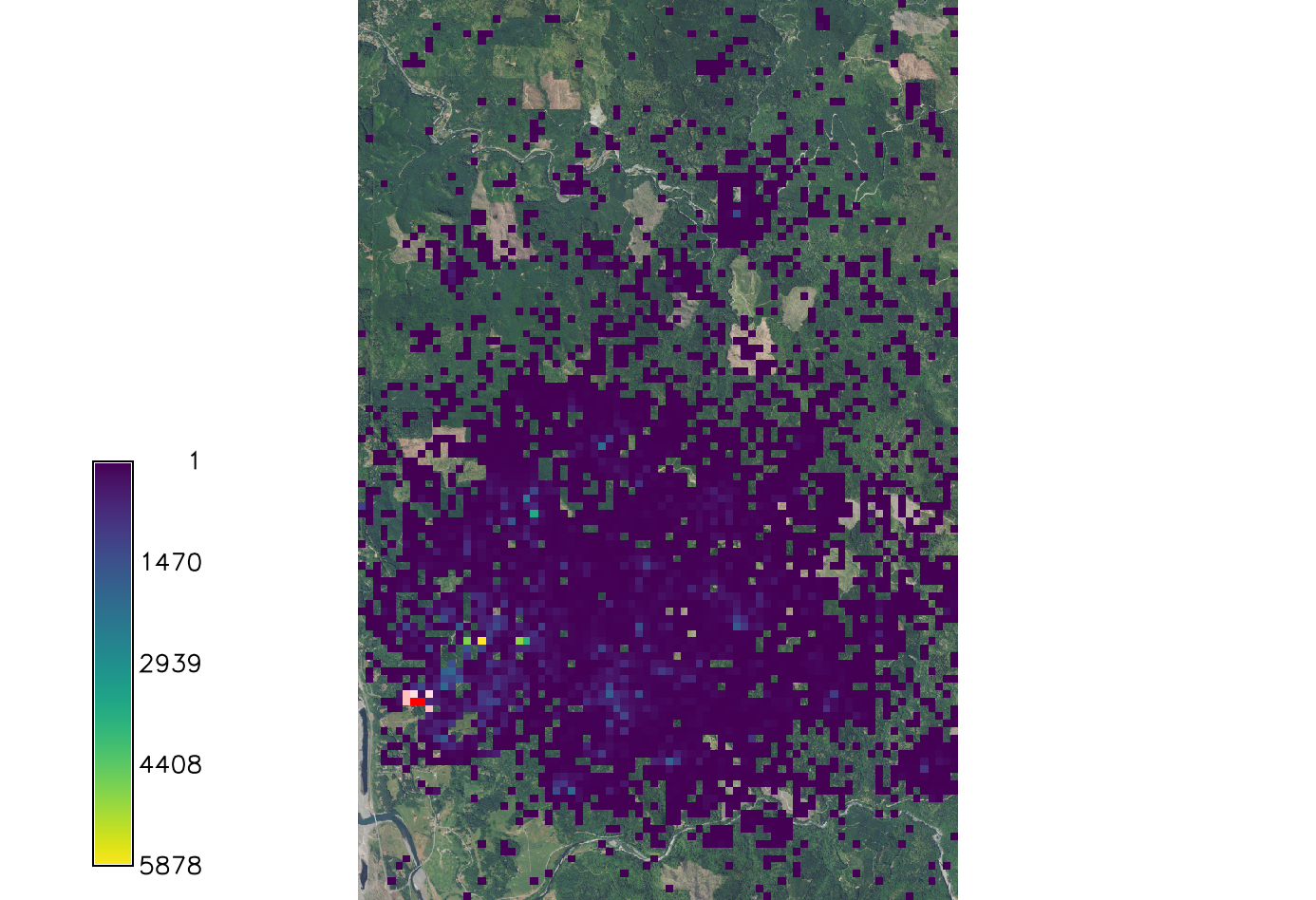
Run the model using the text files created and setting only the required parameters. For this analysis we used a wind direction of NE and are looking at the first 5 years of spread from the initial 2016 infection discovery.
r.spread.sod species=lide_den_int lvtree=all_den_int infected=inf_2016 output=spread_sod wind=NE moisture_file=precipitation.txt temperature_file=temperature.txt start_time=2016 end_time=2021 random_seed=4
Add the initial infected area and ortho photo layers to the display to view the spread. Rearrange layers so ortho is on the bottom.
d.rast inf_2016_null
d.rast ortho
Set all spread values of 0 to null to view orthophoto layer underneath. Then add the layer.
r.null map=spread_sod setnull=0
d.rast spread_sod
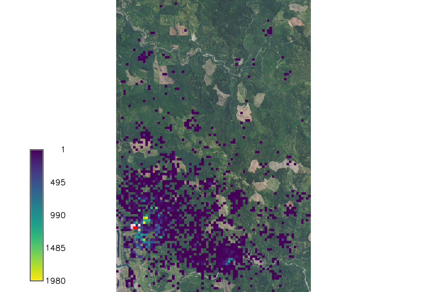
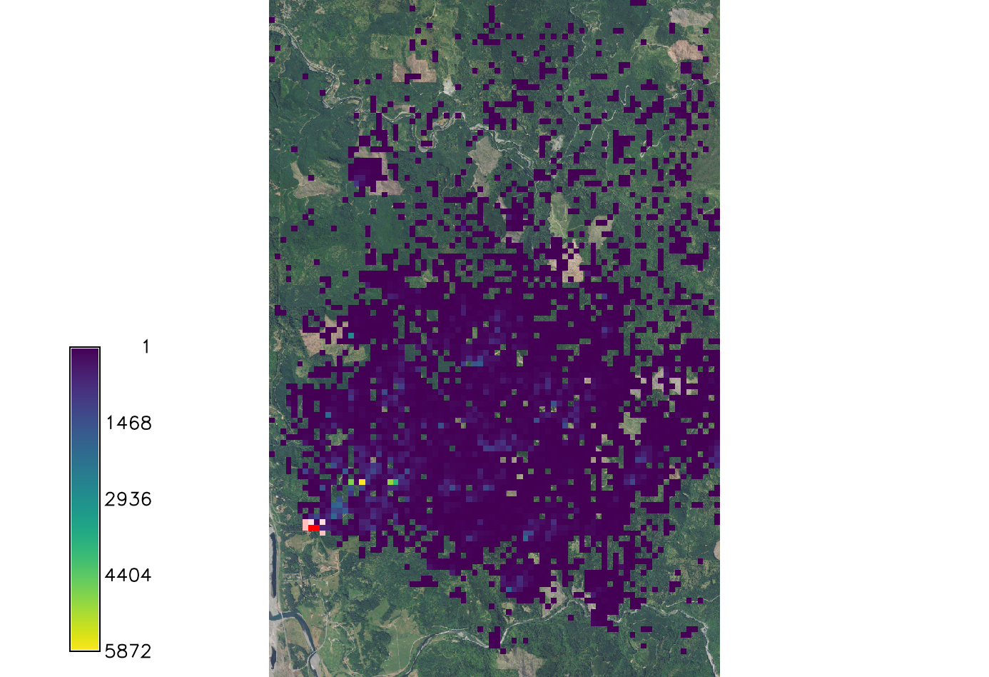
Working with the optional parameters
Kappa(k)
A measure of concentration, a reciprocal measure of dispersion. For this model the Von Mises circular normal distribution equation was used. The default value of k is 2 so the effect wind dispersal has on the spores shows an average distribution.
If k is set to 0 the wind dispersal will have no effect on distribution.
r.spread.sod species=lide_den_int lvtree=all_den_int infected=inf_2016 output=spread_sodk1 wind=NE moisture_file=precipitation.txt temperature_file=temperature.txt start_time=2016 end_time=2021 kappa=0 random_seed=4
If k is larger than 2 the distribution becomes very concentrated around the prevailing wind direction.
r.spread.sod species=lide_den_int lvtree=all_den_int infected=inf_2016 output=spread_sodk2 wind=NE moisture_file=precipitation.txt temperature_file=temperature.txt start_time=2016 end_time=2021 kappa=4 random_seed=4
Gamma(y)
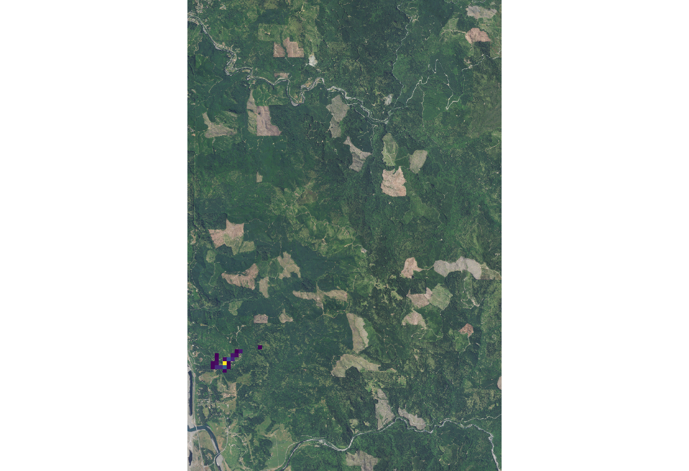
A parameter between 0 and 1 used in the equation for Bernoulli distribution. This parameter is then factored into the Cauchy distribution model for the probability of using the first model. In this instance, a change in the gamma value doesn’t visually affect the output. An example console input for this factor would be:
r.spread.sod species=lide_den_int lvtree=all_den_int infected=inf_2016 output=spread_sodg1 wind=NE moisture_file=precipitation.txt temperature_file=temperature.txt start_time=2016 end_time=2021 gamma=0.5 random_seed=4
Spore_rate
The spore production rate per week for each infected tree. This model uses the Poisson distribution model to determine the spore rate value. At the time of the initial infection the spores were calculated to spread at a rate of 4.4 spores per week.
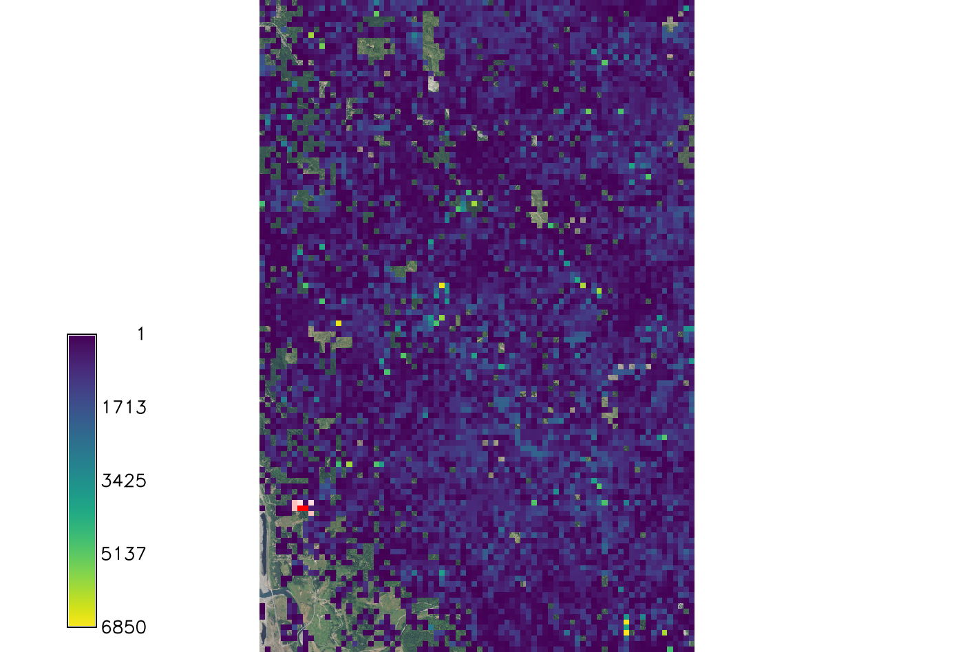
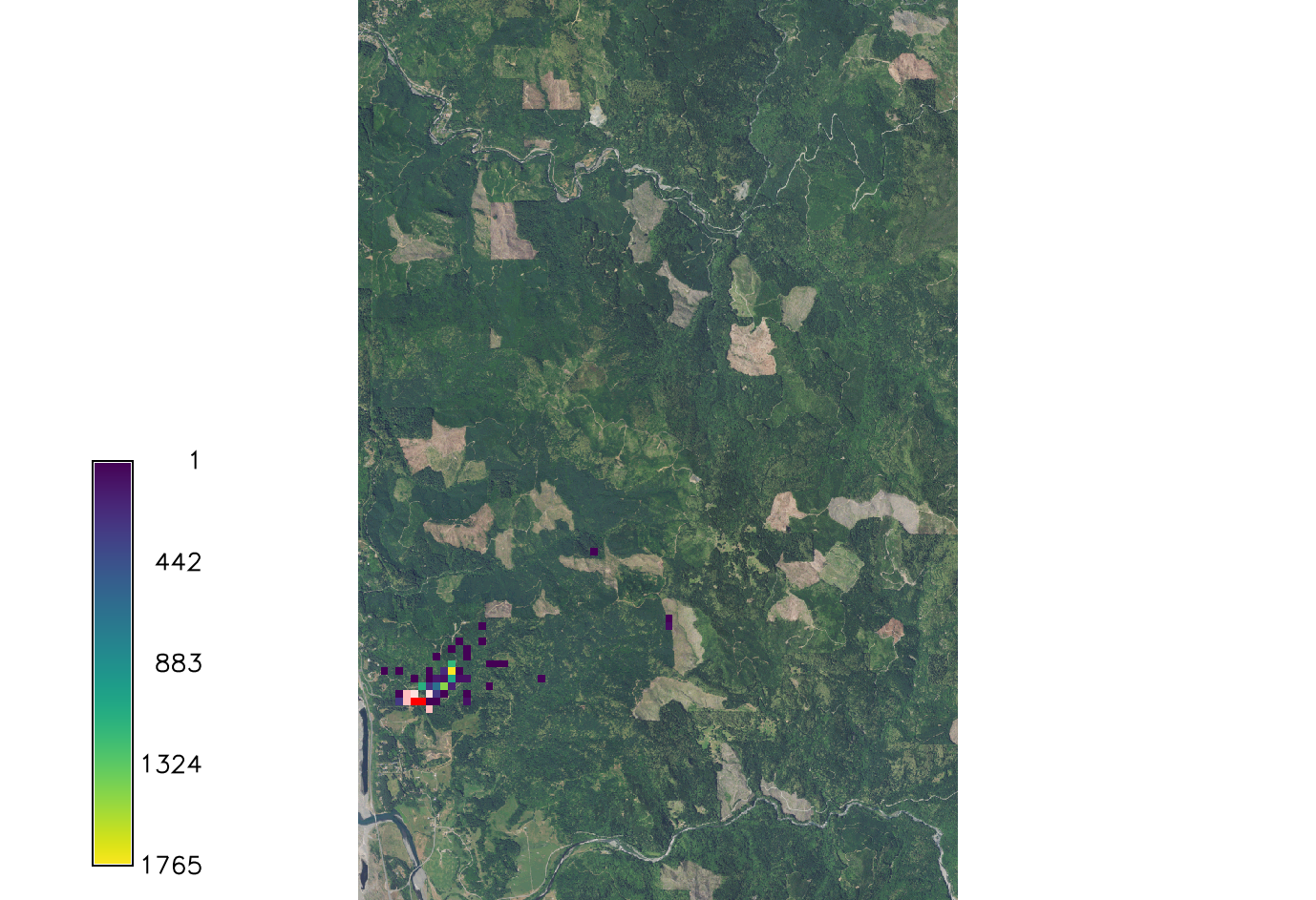
Decreasing the rate down to 1 scales down the spread a great deal. However there are still new areas of spread.
r.spread.sod species=lide_den_int lvtree=all_den_int infected=inf_2016 output=spread_sodsr1 wind=NE moisture_file=precipitation.txt temperature_file=temperature.txt start_time=2016 end_time=2021 spore_rate=1 random_seed=4
Increasing the rate to 10 drastically increases the spread, as to be expected.
r.spread.sod species=lide_den_int lvtree=all_den_int infected=inf_2016 output=spread_sodsr2 wind=NE moisture_file=precipitation.txt temperature_file=temperature.txt start_time=2016 end_time=2021 spore_rate=10 random_seed=4
Updating these calculations on a regular basis can be done quite easily through the model to better monitor the spread. These values can also be adjusted for distinct locations or different forms of sudden oak death.
Scale_1 and Scale_2
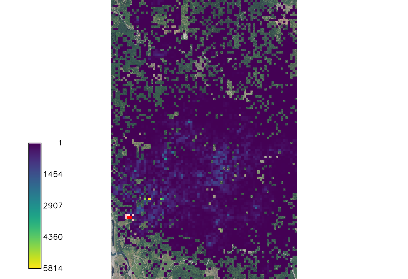
Parameters dealing with the Cauchy distribution, which is the equation that calculates the continuous random distribution of the spores based on inputs. These scale factors effect the outcome by increasing or decreasing the distribution of the spores. Scale_1 is default set to 20.57 which was found to be the initial spread scale in the western Oregon SOD case.
Setting scale_1 factor to 1 so it has no effect in the equation.
r.spread.sod species=lide_den_int lvtree=all_den_int infected=inf_2016 output=spread_sods1_1 wind=NE moisture_file=precipitation.txt temperature_file=temperature.txt start_time=2016 end_time=2021 scale_1=1 random_seed=4
Setting scale_1 factor to 50 so it has a greater effect on the spread.
r.spread.sod species=lide_den_int lvtree=all_den_int infected=inf_2016 output=spread_sods1_2 wind=NE moisture_file=precipitation.txt temperature_file=temperature.txt start_time=2016 end_time=2021 scale_1=50 random_seed=4
Scale_2 is undefined in the equation when the model is run on default. In this instance scale_2 has no visual effect on the output. An example console input for this factor would be:
r.spread.sod species=lide_den_int lvtree=all_den_int infected=inf_2016 output=spread_sods2 wind=NE moisture_file=precipitation.txt temperature_file=temperature.txt start_time=2016 end_time=2021 scale_2=20 random_seed=4