Computational region: Difference between revisions
(+hint about ROI) |
No edit summary |
||
| (5 intermediate revisions by one other user not shown) | |||
| Line 9: | Line 9: | ||
##Raster '''output''' maps have their bounds and resolution equal to those of the current computational region. | ##Raster '''output''' maps have their bounds and resolution equal to those of the current computational region. | ||
##Vector maps are always '''considered completely'''. | ##Vector maps are always '''considered completely'''. | ||
Note that in GRASS, 2D and 3D raster maps share the same region extent. However, the 3D resolution is distinct from the 2D resolution, and they each must be set separately. | |||
'''Hint''' for users migrating from other software packages:<br> | '''Hint''' for users migrating from other software packages:<br> | ||
The current region or computational region can be considered as ''region of interest'' (ROI). | The current region or computational region can be considered as ''region of interest'' (ROI). | ||
=== FAQs | == Understanding the impact of region settings == | ||
It is important to understand the impact of the region settings, notably of resolution, on raster analyses. Both during reprojection from one coordinate system to another, but also for calculating raster statistics with modules such as {{cmd|r.univar}} or {{cmd|v.rast.stats}}, the values of your raster pixels can be modified depending on your region settings and thus modify the results of any analysis. | |||
If a raster map has an original resolution that is different from the resolution of the current computational region, but also when the current computational region's cells are shifted in space compared to the original raster map, the values are resampled on-the-fly by GRASS GIS, using the nearest neighbor method (see some of the details in the [https://grass.osgeo.org/grass70/manuals/rasterintro.html#raster-map-operations Raster introduction manual]. | |||
The nature of the impact depends on the nature of the data. If the data represents a continuous field, but not absolute values that depends on the size of the space, then nearest neighbor resampling might slightly alter your data, but not fundamentally. Examples of continuous field data are elevation, average rainfall, concentration of pollutants in soil, water or air, land surface reflectance (satellite imagery), etc. Examples of absolute values are number of inhabitants, total rainfall per pixel, total turnover of enterprises, etc. | |||
=== Continuous field data === | |||
When continuous field data is resampled, the challenge is to estimate the values of that continuous field at points where these values are not known. This is a classical interpolation problem. Which interpolation technique is best depends on the data and on the desired output. If nearest neighbor resampling is not sufficient, several GRASS GIS modules offer other options. See [[Interpolation]] wiki page and the above-mentioned raster introduction manual for more details. | |||
=== Absolute values data === | |||
Absolute data is different. Here the challenge is to redistribute a finite amount of something into the new cells. It is not an issue of interpolation, but an issue of reassigning data from one partition into another. | |||
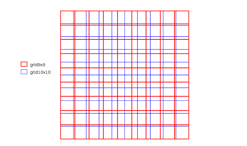
As an example, imagine a simple map of population which is 10 rows and 10 columns. In this map the population in each pixel is 1. Imagine also a computational region with the same extent but of 9 rows and 9 columns. Cells in the computational region are thus slightly bigger than cells in the original raster map, and there are 100 cells in the map, but only 81 cells in the region. | |||
[[Image:Grid_examples.png|350px|center|thumb|Grid representation of the two raster cell settings: 9x9 and 10x10 within the same spatial extent]] | |||
The automatic, on-the-fly nearest neighbor resampling will thus pick the 81 cells in the raster map whose centers are closest to the centers of the cells in the computational regions and affect the values of these cells to the resampling output. In other words, the values of 19 cells are "lost". When you now calculate the sum of the values with {{cmd|r.univar}} the result will be different than if you adjust the computational region to the original map: | |||
<source lang="bash"> | |||
g.region s=0 n=10 w=0 e=10 res=1 -p | |||
[...] | |||
north: 10 | |||
south: 0 | |||
west: 0 | |||
east: 10 | |||
nsres: 1 | |||
ewres: 1 | |||
rows: 10 | |||
cols: 10 | |||
[...] | |||
r.mapcalc "tenbyten = 1" | |||
r.univar tenbyten | |||
[...] | |||
sum: 100 | |||
g.region cols=9 rows=9 -p | |||
[...]north: 10 | |||
south: 0 | |||
west: 0 | |||
east: 10 | |||
nsres: 1.11111111 | |||
ewres: 1.11111111 | |||
rows: 9 | |||
cols: 9 | |||
[...] | |||
r.univar tenbyten | |||
[...] | |||
sum: 81 | |||
</source> | |||
In order to get the original total, you will have to do other types of resampling, notably using {{cmd|r.resamp.stats}} or possibly {{cmd|r.resamp.interp}}. For example (still using the 9x9 region): | |||
<source lang="bash"> | |||
r.resamp.stats in=tenbyten out=ninebynine_sum method=sum | |||
r.univar ninebynine_sum | |||
[...] | |||
n: 81 | |||
minimum: 1 | |||
maximum: 4 | |||
[...] | |||
mean: 1.23457 | |||
[...] | |||
sum: 100 | |||
</source> | |||
Or, to assign values depending on the share of each original cell falling into the region's cell: | |||
<source lang="bash"> | |||
r.resamp.stats -w in=tenbyten out=ninebynine_weighted_sum method=sum | |||
r.univar ninebynine_weighted_sum | |||
[...] | |||
n: 81 | |||
minimum: 1.23457 | |||
maximum: 1.23457 | |||
[...] | |||
mean: 1.23457 | |||
[...] | |||
sum: 100 | |||
</source> | |||
For more details about the interpolation methods, see [[Interpolation]] and the [https://grass.osgeo.org/grass70/manuals/rasterintro.html#raster-map-operations Raster introduction manual]. | |||
== FAQs == | |||
'''Q:''' I don't see anything! | '''Q:''' I don't see anything! | ||
Latest revision as of 19:37, 2 June 2025
The current region or computational region is the actual setting of the region boundaries and the actual raster resolution.
As a general rule in GRASS:
- Raster maps are always imported completely at their own resolution (exception: WMS imported layers).
- Vector maps are always imported completely.
- In computations,
- raster input maps are automatically cropped/padded and rescaled (using nearest neighbour resampling) to match the current region in order to produce the output raster map or to query values.
- Raster output maps have their bounds and resolution equal to those of the current computational region.
- Vector maps are always considered completely.
Note that in GRASS, 2D and 3D raster maps share the same region extent. However, the 3D resolution is distinct from the 2D resolution, and they each must be set separately.
Hint for users migrating from other software packages:
The current region or computational region can be considered as region of interest (ROI).
Understanding the impact of region settings
It is important to understand the impact of the region settings, notably of resolution, on raster analyses. Both during reprojection from one coordinate system to another, but also for calculating raster statistics with modules such as r.univar or v.rast.stats, the values of your raster pixels can be modified depending on your region settings and thus modify the results of any analysis.
If a raster map has an original resolution that is different from the resolution of the current computational region, but also when the current computational region's cells are shifted in space compared to the original raster map, the values are resampled on-the-fly by GRASS GIS, using the nearest neighbor method (see some of the details in the Raster introduction manual.
The nature of the impact depends on the nature of the data. If the data represents a continuous field, but not absolute values that depends on the size of the space, then nearest neighbor resampling might slightly alter your data, but not fundamentally. Examples of continuous field data are elevation, average rainfall, concentration of pollutants in soil, water or air, land surface reflectance (satellite imagery), etc. Examples of absolute values are number of inhabitants, total rainfall per pixel, total turnover of enterprises, etc.
Continuous field data
When continuous field data is resampled, the challenge is to estimate the values of that continuous field at points where these values are not known. This is a classical interpolation problem. Which interpolation technique is best depends on the data and on the desired output. If nearest neighbor resampling is not sufficient, several GRASS GIS modules offer other options. See Interpolation wiki page and the above-mentioned raster introduction manual for more details.
Absolute values data
Absolute data is different. Here the challenge is to redistribute a finite amount of something into the new cells. It is not an issue of interpolation, but an issue of reassigning data from one partition into another.
As an example, imagine a simple map of population which is 10 rows and 10 columns. In this map the population in each pixel is 1. Imagine also a computational region with the same extent but of 9 rows and 9 columns. Cells in the computational region are thus slightly bigger than cells in the original raster map, and there are 100 cells in the map, but only 81 cells in the region.

The automatic, on-the-fly nearest neighbor resampling will thus pick the 81 cells in the raster map whose centers are closest to the centers of the cells in the computational regions and affect the values of these cells to the resampling output. In other words, the values of 19 cells are "lost". When you now calculate the sum of the values with r.univar the result will be different than if you adjust the computational region to the original map:
g.region s=0 n=10 w=0 e=10 res=1 -p
[...]
north:      10
south:      0
west:       0
east:       10
nsres:      1
ewres:      1
rows:       10
cols:       10
[...]

r.mapcalc "tenbyten = 1"

r.univar tenbyten
[...]
sum: 100

g.region cols=9 rows=9 -p
[...]north:      10
south:      0
west:       0
east:       10
nsres:      1.11111111
ewres:      1.11111111
rows:       9
cols:       9
[...]

r.univar tenbyten
[...]
sum: 81
In order to get the original total, you will have to do other types of resampling, notably using r.resamp.stats or possibly r.resamp.interp. For example (still using the 9x9 region):
r.resamp.stats in=tenbyten out=ninebynine_sum method=sum
r.univar ninebynine_sum
[...]
n: 81
minimum: 1
maximum: 4
[...]
mean: 1.23457
[...]
sum: 100
Or, to assign values depending on the share of each original cell falling into the region's cell:
r.resamp.stats -w in=tenbyten out=ninebynine_weighted_sum method=sum
r.univar ninebynine_weighted_sum
[...]
n: 81
minimum: 1.23457
maximum: 1.23457
[...]
mean: 1.23457
[...]
sum: 100
For more details about the interpolation methods, see Interpolation and the Raster introduction manual.
FAQs
Q: I don't see anything!
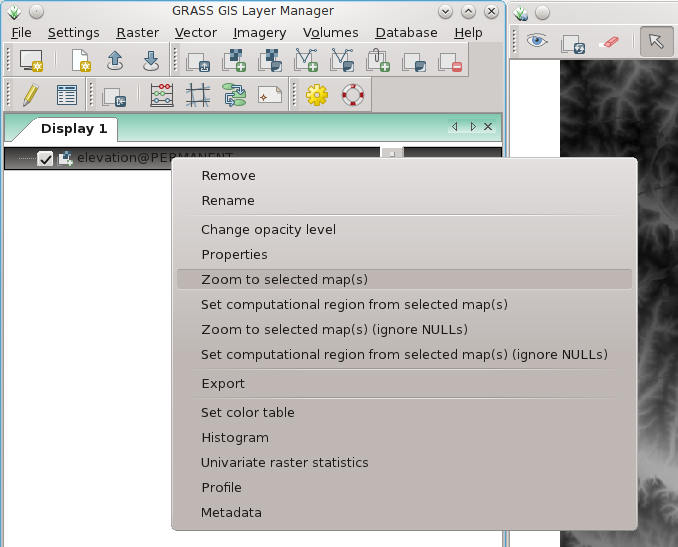
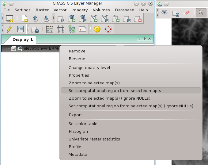
A: Typically the computational region is set to an area not covering the raster map of interest. Use g.region to adjust the computational region settings, e.g. by setting it to the raster map:
g.region rast=myrastermap -p
Using the graphical user interface:
Set display to selected map:

Set computational region to selected map:

Q: The resolution of my region is not the one I asked for!
A: Sometimes, the resolution of the computational region is not matching exactly the resolution entered to g.region. Here's an example:
g.region rast=myrastermap res=1 -p
(...)
nsres:      0.9993515
ewres:      1.00025576
(...)
To force the computational region to match the resolution entered, you need to use the -a flag:
g.region rast=myrastermap res=1 -ap
(...)
nsres:      1
ewres:      1
(...)
Q: The raster map looks ugly.
A: The resolution of the computational region does not match the resolution of the raster map. Use g.region to adjust the resolution settings of the computational region or set it to the raster map (see above).
Q: I get "xyz module: G_malloc error"
A: You likely try to use more memory than your computer offers which is commonly caused by a too high raster resolution (or too large computational region). E.g., it is pointless to calculate common DEM data at nanometer raster resolution. Set the region extent and raster resolution properly with g.region (in the wxGUI: menu Settings -> Region -> Display Region | Set Region).
Q: I want to subset a raster map!
A: While this is done on the fly by setting the computational region properly, you can still create a subset raster map copy with
r.mapcalc "subset = original_map"