Image classification: Difference between revisions
(+ Background information concerning {{cmd|i.cluster}}) |
m (remove hardcoded version specific urls, use latest version) |
||
| (14 intermediate revisions by 3 users not shown) | |||
| Line 6: | Line 6: | ||
| ||'''radiometric<BR>unsupervised'''||'''radiometric<BR>supervised 1'''||'''radiometric<BR>supervised 2'''||'''radiometric & geometric<BR>supervised''' | | ||'''radiometric<BR>unsupervised'''||'''radiometric<BR>supervised 1'''||'''radiometric<BR>supervised 2'''||'''radiometric & geometric<BR>supervised''' | ||
|- | |- | ||
| '''Image Preprocessing''' || colspan="4" style="text-align: center;"| {{AddonCmd|r.seg}} (optional, in case of noisy original data) | | '''Image Preprocessing''' || colspan="4" style="text-align: center;"| {{AddonCmd|r.smooth.seg}} (optional, in case of noisy original data) | ||
|- | |- | ||
| '''Preprocessing'''||{{cmd|i.cluster}}||{{cmd|i.class}} (monitor digitizing), {{cmd|g.gui.iclass | | '''Segmentation''' || colspan="4" style="text-align: center;"| {{cmd|i.segment}} | ||
|- | |||
| '''Preprocessing'''||{{cmd|i.cluster}}||{{cmd|i.class}} (monitor digitizing), {{cmd|g.gui.iclass}} (in GRASS 70)||{{cmd|i.gensig}} (using training maps)||{{cmd|i.gensigset}} (using training maps) | |||
|- | |- | ||
| '''Classification'''||{{cmd|i.maxlik}}||{{cmd|i.maxlik}}||{{cmd|i.maxlik}}||{{cmd|i.smap}} | | '''Classification'''||{{cmd|i.maxlik}}||{{cmd|i.maxlik}}||{{cmd|i.maxlik}}||{{cmd|i.smap}} | ||
| Line 19: | Line 21: | ||
You can digitize training areas with either r.digit (not recommended) or <strike>v.digit</strike> [[GRASS Digitizing tool]] + v.to.rast (recommended) | You can digitize training areas with either r.digit (not recommended) or <strike>v.digit</strike> [[GRASS Digitizing tool]] + v.to.rast (recommended) | ||
=== Image Preprocessing (optional) === | === Image Preprocessing (optional) === | ||
* {{AddonCmd|r.seg}} - produces a smooth approximation of the data and performs discontinuity detection. The module is based on the Mumford-Shah variational model for image segmentation. Used as pre-analysis for a subsequent classification. | * {{AddonCmd|r.smooth.seg}} - produces a smooth approximation of the data and performs discontinuity detection. The module is based on the Mumford-Shah variational model for image segmentation. Used as pre-analysis for a subsequent classification. | ||
: For details, see the | : For details, see the {{AddonCmd|r.smooth.seg}} manual (formerly called: r.seg) | ||
* {{cmd|i.segment}} - identifies segments (objects) from imagery data based (currently) on a region growing and merging algorithm. The image segmentation results can be useful (on their own or) as a preprocessing step for image classification, i.e. reduce noise and speed up the classification. | * {{cmd|i.segment}} - identifies segments (objects) from imagery data based (currently) on a region growing and merging algorithm. The image segmentation results can be useful (on their own or) as a preprocessing step for image classification, i.e. reduce noise and speed up the classification. | ||
** Classification of these segments: see below in "Unsupervised classification". | |||
=== Interactive setup === | === Interactive setup === | ||
| Line 30: | Line 32: | ||
* {{cmd|i.class}} - Generates spectral signatures for an image by allowing the user to outline regions of interest. | * {{cmd|i.class}} - Generates spectral signatures for an image by allowing the user to outline regions of interest. | ||
: The resulting signature file can be used as input for {{cmd|i.maxlik}} or as a seed signature file for {{cmd|i.cluster}}. | : The resulting signature file can be used as input for {{cmd|i.maxlik}} or as a seed signature file for {{cmd|i.cluster}}. | ||
* {{cmd|g.gui.iclass | * {{cmd|g.gui.iclass}} - Tool for supervised classification of imagery data. | ||
=== Preprocessing === | === Preprocessing === | ||
| Line 41: | Line 43: | ||
Background information concerning {{cmd|i.cluster}}: | Background information concerning {{cmd|i.cluster}}: | ||
* Discussion: [https://lists.osgeo.org/pipermail/grass-user/2012-October/066046.html Is "i.cluster" an implementation of the ISODATA algorithm?] | * Discussion: [https://lists.osgeo.org/pipermail/grass-user/2012-October/066046.html Is "i.cluster" an implementation of the ISODATA algorithm?] | ||
* [User:NikosA/About Clustering About Clustering] | * [[User:NikosA/About Clustering|About Clustering]] | ||
=== Unsupervised classification === | === Unsupervised classification === | ||
| Line 50: | Line 52: | ||
: Classification is based on the spectral signature information generated by {{cmd|i.cluster}} (see above) | : Classification is based on the spectral signature information generated by {{cmd|i.cluster}} (see above) | ||
* GRASS GIS 7: {{cmd|i.segment}} | * GRASS GIS 7: {{cmd|i.segment}} | ||
** Classification of these segments could be achieved with these addons: {{AddonCmd|v.class.mlR}}, {{AddonCmd|v.class.mlpy}}, {{AddonCmd|v.class.ml}}. | |||
See example below. | See example below. | ||
| Line 59: | Line 62: | ||
* {{cmd|g.gui.iclass}} - Tool for supervised classification of imagery data. | * {{cmd|g.gui.iclass}} - Tool for supervised classification of imagery data. | ||
* {{cmd|i.smap}} - Performs contextual (image segmentation) image classification using sequential maximum a posteriori (SMAP) estimation. | * {{cmd|i.smap}} - Performs contextual (image segmentation) image classification using sequential maximum a posteriori (SMAP) estimation. | ||
* {{AddonCmd|r.learn.ml}} - Supervised Machine Learning classification and regression of GRASS rasters using the python scikit-learn package | |||
* In case of panchromatic maps or limited amount of channels, it is often recommended to generate synthetic channels through texture analysis ({{cmd|r.texture}}) | * In case of panchromatic maps or limited amount of channels, it is often recommended to generate synthetic channels through texture analysis ({{cmd|r.texture}}) | ||
See example below. | See example below. | ||
== Object-based classification and image segmentation == | |||
''Created based on [http://lists.osgeo.org/pipermail/grass-user/2014-June/070384.html Summary of object-based classification possibilities in GRASS GIS (June 2014)]. Feel free to merge this with other content or with different page.'' | |||
Related commands: | |||
* {{cmd|i.segment}} - Identifies segments (objects) from imagery data. | |||
* {{AddonCmd|i.segment.hierarchical}} performs a hierarchical segmentation on an image (group). The module uses internally {{cmd|i.segment}} | |||
* {{AddonCmd|i.segment.stats}} calculates statistics describing raster area. | |||
* extra: {{AddonCmd|r.smooth.seg}} - Generates a piece-wise smooth approximation of the input raster and a discontinuity map. | |||
* extra: {{AddonCmd|i.superpixels.slic}} - Perform image segmentation using the SLIC segmentation method. | |||
Background information: | |||
* '''Publications''' on [https://scholar.google.fr/scholar?as_sdt=1%2C5&as_ylo=2014&as_vis=1&q=grass+gis+obia&btnG= GRASS GIS and Object Based Image Analysis (OBIA) techniques] (via Google Scholar) | |||
* Old references | |||
** [http://lists.osgeo.org/pipermail/grass-dev/2013-October/066181.html Moritz's steps and the main discussion: Object-based image classification in GRASS] ([http://osgeo-org.1560.x6.nabble.com/Object-based-image-classification-in-GRASS-td5086693.html nabble link]) | |||
** [http://geo.fsv.cvut.cz/gwiki/153ZODH_/_15._cvi%C4%8Den%C3%AD Moritz's steps in a nice guide by Martin, in Czech with images] ([http://translate.google.com/translate?sl=cs&tl=en&js=n&prev=_t&hl=en&ie=UTF-8&u=http%3A%2F%2Fgeo.fsv.cvut.cz%2Fgwiki%2F153ZODH_%2F_15._cvi%25C4%258Den%25C3%25AD&act=url English Google-translation]) | |||
** [http://lists.osgeo.org/pipermail/grass-user/2013-November/069254.html Alternative notes by Moritz: Classification of segments] ([http://osgeo-org.1560.x6.nabble.com/Re-Classification-of-segments-td5088837.html nabble link]) | |||
** [http://lists.osgeo.org/pipermail/grass-dev/2014-January/066804.html Pietro's steps and tools] ([http://osgeo-org.1560.x6.nabble.com/Object-based-image-classification-in-GRASS-tp5086693p5096826.html nabble link]) | |||
* [http://lists.osgeo.org/pipermail/grass-dev/2013-August/065287.html Another discussion about what variables to use: Object-based classification] ([http://osgeo-org.1560.x6.nabble.com/i-segment-invalid-region-id-0-tp5066102p5070201.html nabble link]) | |||
Source code and scripts: | |||
* The source code of the classification tools (for inspiration in writing your own scripts): | |||
** v.class.ml: http://svn.osgeo.org/grass/grass-addons/grass7/vector/v.class.ml/ (Pietro's tool) | |||
** v.class.mlpy: http://svn.osgeo.org/grass/grass-addons/grass7/vector/v.class.mlpy/ (Vaclav's tool) | |||
** i.mlpy.py: http://svn.osgeo.org/grass/sandbox/turek/i.mlpy.py (Stepan's tool) | |||
* List of Python machine learning libraries: | |||
** scikit-learn, http://scikit-learn.org/ (used by v.class.ml) | |||
** mlpy, http://mlpy.sourceforge.net/ (used by v.class.ml, v.class.mlpy and i.mlpy) | |||
** Pandas, http://pandas.pydata.org/ | |||
** Milk, http://luispedro.org/software/milk | |||
== Small classification tutorial == | == Small classification tutorial == | ||
| Line 261: | Line 295: | ||
== | == Assessing the quality and result of the classification == | ||
* | * {{cmd|r.cross}} | ||
* {{cmd|r.kappa}} | |||
* {{AddonCmd|r.change.info}}: Landscape change assessment | |||
* | |||
* | |||
== Further reading on classification with GRASS GIS == | |||
== Further reading classification with GRASS == | * Georganos, S., Lennert, M., Grippa, T., Vanhuysse, S., Johnson, B., Wolff, E., 2018. Normalization in Unsupervised Segmentation Parameter Optimization: A Solution Based on Local Regression Trend Analysis. Remote Sensing 10, 222. https://doi.org/10.3390/rs10020222 | ||
* Micha Silver: [ | * Grippa, T., Lennert, M., Beaumont, B., Vanhuysse, S., Stephenne, N., Wolff, E., 2017. An Open-Source Semi-Automated Processing Chain for Urban Object-Based Classification. Remote Sensing 9, 358. https://doi.org/10.3390/rs9040358 | ||
* Beaumont, B., Grippa, T., Lennert, M., Vanhuysse, S.G., Stephenne, N.R., Wolff, E., 2017. Toward an operational framework for fine-scale urban land-cover mapping in Wallonia using submeter remote sensing and ancillary vector data. JARS, JARSC4 11, 036011. https://doi.org/10.1117/1.JRS.11.036011 | |||
* Micha Silver: [https://www.surfaces.co.il/analyzing-acacia-tree-health-in-the-arava-with-grass-gis/ Analyzing acacia tree health in the Arava with GRASS GIS] | |||
* Perrygeo: [http://www.perrygeo.net/wordpress/?p=104 Impervious surface deliniation with GRASS] | * Perrygeo: [http://www.perrygeo.net/wordpress/?p=104 Impervious surface deliniation with GRASS] | ||
* Dylan Beaudette: [http://casoilresource.lawr.ucdavis.edu/drupal/node/159 Working with Landsat Data] | * Dylan Beaudette: [http://casoilresource.lawr.ucdavis.edu/drupal/node/159 Working with Landsat Data] | ||
* Dylan Beaudette: [http://casoilresource.lawr.ucdavis.edu/drupal/node/548 Canopy Quantification via Image Classification] | * Dylan Beaudette: [http://casoilresource.lawr.ucdavis.edu/drupal/node/548 Canopy Quantification via Image Classification] | ||
* [http://istgeo.ist.supsi.ch/site/node/24 Segmentazione o classificazione d'immagini con GRASS] (in italiano) | * [http://istgeo.ist.supsi.ch/site/node/24 Segmentazione o classificazione d'immagini con GRASS] (in italiano) | ||
* Di Palma, F.; Amato, F.; Nolè, G.; Martellozzo, F.; Murgante, B. 2016: A SMAP Supervised Classification of Landsat Images for Urban Sprawl Evaluation. ISPRS Int. J. Geo-Inf. 2016, 5, 109. PDF: http://www.mdpi.com/2220-9964/5/7/109 | |||
== Further reading on OBIA with GRASS GIS == | |||
* A complete toolchain for object-based image analysis with GRASS GIS | |||
** Abstract: https://frab.fossgis-konferenz.de/en/foss4g-2016/public/events/1289 | |||
** Video: https://av.tib.eu/media/20409 | |||
** Software: https://github.com/tgrippa/Opensource_OBIA_processing_chain | |||
[[Category: Documentation]] | [[Category: Documentation]] | ||
[[Category: Tutorial]] | [[Category: Tutorial]] | ||
[[Category: Image processing]] | [[Category: Image processing]] | ||
Latest revision as of 10:48, 4 December 2018
Image classification
Classification methods in GRASS
| radiometric unsupervised |
radiometric supervised 1 |
radiometric supervised 2 |
radiometric & geometric supervised | |
| Image Preprocessing | r.smooth.seg (optional, in case of noisy original data) | |||
| Segmentation | i.segment | |||
| Preprocessing | i.cluster | i.class (monitor digitizing), g.gui.iclass (in GRASS 70) | i.gensig (using training maps) | i.gensigset (using training maps) |
| Classification | i.maxlik | i.maxlik | i.maxlik | i.smap |
| Remarks | automated run based | requires digitalization | requires digitalization | requires digitalization |
| on image statistics | of training areas | of training areas | of training areas | |
You can digitize training areas with either r.digit (not recommended) or v.digit GRASS Digitizing tool + v.to.rast (recommended)
Image Preprocessing (optional)
- r.smooth.seg - produces a smooth approximation of the data and performs discontinuity detection. The module is based on the Mumford-Shah variational model for image segmentation. Used as pre-analysis for a subsequent classification.
- For details, see the r.smooth.seg manual (formerly called: r.seg)
- i.segment - identifies segments (objects) from imagery data based (currently) on a region growing and merging algorithm. The image segmentation results can be useful (on their own or) as a preprocessing step for image classification, i.e. reduce noise and speed up the classification.
- Classification of these segments: see below in "Unsupervised classification".
Interactive setup
- i.class - Generates spectral signatures for an image by allowing the user to outline regions of interest.
- The resulting signature file can be used as input for i.maxlik or as a seed signature file for i.cluster.
- g.gui.iclass - Tool for supervised classification of imagery data.
Preprocessing
- i.cluster - Generates spectral signatures for land cover types in an image using a clustering algorithm.
- The resulting signature file is used as input for i.maxlik, to generate an unsupervised image classification.
- i.gensig - Generates statistics for i.maxlik from raster map layer.
- i.gensigset - Generate statistics for i.smap from raster map layer.
Background information concerning i.cluster:
Unsupervised classification
For an introduction, see for example Cluster_analysis.
- i.maxlik - Classifies the cell spectral reflectances in imagery data.
- Classification is based on the spectral signature information generated by i.cluster (see above)
- GRASS GIS 7: i.segment
- Classification of these segments could be achieved with these addons: v.class.mlR, v.class.mlpy, v.class.ml.
See example below.
Supervised classification
- i.maxlik - Classifies the cell spectral reflectances in imagery data.
- Classification is based on the spectral signature information generated by either i.class, or i.gensig.
- g.gui.iclass - Tool for supervised classification of imagery data.
- i.smap - Performs contextual (image segmentation) image classification using sequential maximum a posteriori (SMAP) estimation.
- r.learn.ml - Supervised Machine Learning classification and regression of GRASS rasters using the python scikit-learn package
- In case of panchromatic maps or limited amount of channels, it is often recommended to generate synthetic channels through texture analysis (r.texture)
See example below.
Object-based classification and image segmentation
Created based on Summary of object-based classification possibilities in GRASS GIS (June 2014). Feel free to merge this with other content or with different page.
Related commands:
- i.segment - Identifies segments (objects) from imagery data.
- i.segment.hierarchical performs a hierarchical segmentation on an image (group). The module uses internally i.segment
- i.segment.stats calculates statistics describing raster area.
- extra: r.smooth.seg - Generates a piece-wise smooth approximation of the input raster and a discontinuity map.
- extra: i.superpixels.slic - Perform image segmentation using the SLIC segmentation method.
Background information:
- Publications on GRASS GIS and Object Based Image Analysis (OBIA) techniques (via Google Scholar)
- Old references
- Another discussion about what variables to use: Object-based classification (nabble link)
Source code and scripts:
- The source code of the classification tools (for inspiration in writing your own scripts):
- v.class.ml: http://svn.osgeo.org/grass/grass-addons/grass7/vector/v.class.ml/ (Pietro's tool)
- v.class.mlpy: http://svn.osgeo.org/grass/grass-addons/grass7/vector/v.class.mlpy/ (Vaclav's tool)
- i.mlpy.py: http://svn.osgeo.org/grass/sandbox/turek/i.mlpy.py (Stepan's tool)
- List of Python machine learning libraries:
- scikit-learn, http://scikit-learn.org/ (used by v.class.ml)
- mlpy, http://mlpy.sourceforge.net/ (used by v.class.ml, v.class.mlpy and i.mlpy)
- Pandas, http://pandas.pydata.org/
- Milk, http://luispedro.org/software/milk
Small classification tutorial
Required: GRASS >= 6.4
We are using Landsat satellite data prepared for the North Carolina sampling site. It is a multispectral dataset where each channel is stored in a separate map.
We are using the North Carolina location here.
Warming up with Landsat TM
 # look what maps are there
 g.list rast
 # set to one of the color channels and print current region settings
 g.region rast=lsat7_2002_10 -p
 # look at some Landsat map (1: blue, 2: green, 3: red, 4: near infrared etc.)
 d.mon x0
 d.rast lsat7_2002_10
 d.rast lsat7_2002_20
 d.rast lsat7_2002_30
 d.rast lsat7_2002_40
We can easily query the spectrum for individual points:
d.what.rast lsat7_2002_10,lsat7_2002_20,lsat7_2002_30,lsat7_2002_40
Histogram of a channel:
d.histogram lsat7_2002_10
Create RGB view on the fly, true and false color:
 d.rgb b=lsat7_2002_10 g=lsat7_2002_20 r=lsat7_2002_30
 d.rgb b=lsat7_2002_70 g=lsat7_2002_20 r=lsat7_2002_30
 d.rgb b=lsat7_2002_70 g=lsat7_2002_50 r=lsat7_2002_30
 d.rgb b=lsat7_2002_70 g=lsat7_2002_50 r=lsat7_2002_10
Check thermal channel (encoded to fit into 0.255 data range):
- http://landsathandbook.gsfc.nasa.gov/handbook/handbook_htmls/chapter11/chapter11.html
- Look up LMIN/LMAX: "Table 11.2 ETM+ Spectral Radiance Range watts/(meter squared * ster * µm)"
- we won't go into details here, r.mapcalc would be used to convert to Kelvoin/degree Celsius.
 # look at encoded thermal channel
 d.rast lsat7_2002_61
NDVI as example for map algebra:
 r.mapcalc "ndvi = 1.0 * (lsat7_2002_40 - lsat7_2002_30)/(lsat7_2002_40 + lsat7_2002_30)"
 d.rast.leg ndvi
 r.colors ndvi color=ndvi
 d.rast.leg ndvi
Show selected NDVI "classes":
 d.rast ndvi val=0.3-1.0
 d.rast ndvi val=-1.0--0.1
 d.rast ndvi val=0.0-0.2
 d.rast ndvi val=0.0-0.3
Look at panchromatic channel, compare resolution:
 g.region rast=lsat7_2002_80 -p
 d.erase -f
 d.rast lsat7_2002_80
 d.zoom
 d.rast lsat7_2002_30
 d.rast lsat7_2002_80
Image Classification
Set region setting to red image:
g.region rast=lsat7_2002_30 -p
Create a group
 i.group group=lsat7_2002 subgroup=lsat7_2002 \
   input=lsat7_2002_10,lsat7_2002_20,lsat7_2002_30,lsat7_2002_40,lsat7_2002_50,lsat7_2002_70
Unsupervised classification
Generate unsupervised statistics
i.cluster group=lsat7_2002 subgroup=lsat7_2002 sigfile=lsat7_2002_sig classes=10 reportfile=lsat7_2002.txt
 # look at report file
 gedit lsat7_2002.txt
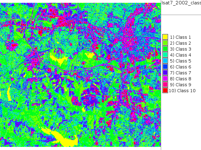
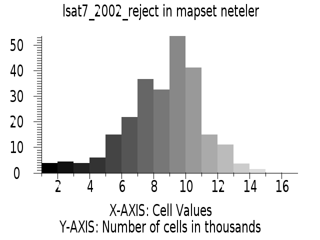
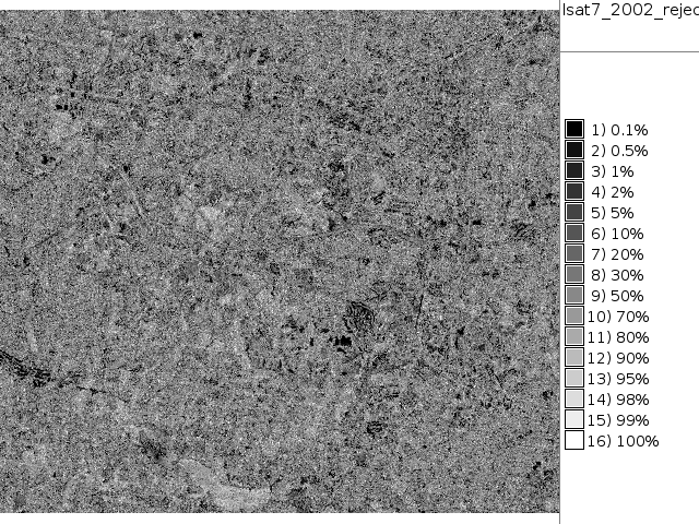
Assign pixels to classes, check quality of assignment:
i.maxlik group=lsat7_2002 subgroup=lsat7_2002 sigfile=lsat7_2002_sig class=lsat7_2002_class reject=lsat7_2002_reject
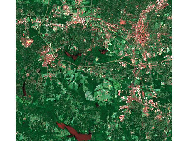
 # false color composite
 d.mon x0 ; d.font Vera
 d.rgb b=lsat7_2002_70 g=lsat7_2002_50 r=lsat7_2002_10
 # classification result
 d.mon x1 ; d.font Vera
 d.rast.leg lsat7_2002_class
 # rejection map
 d.mon x2 ; d.font Vera
 d.rast.leg lsat7_2002_reject
 # rejection histogram
 d.mon x3 ; d.font Vera
 d.histogram lsat7_2002_reject
 |
 |
 |
 |
Play with different cluster separations:
 i.cluster group=lsat7_2002 subgroup=lsat7_2002 sigfile=lsat7_2002_sig classes=10 reportfile=lsat7_2002.txt separation=1.5
 i.maxlik group=lsat7_2002 subgroup=lsat7_2002 sigfile=lsat7_2002_sig class=lsat7_2002_class2 reject=lsat7_2002_reject2
 d.mon x4
 d.rast.leg lsat7_2002_class2
 d.rast.leg lsat7_2002_reject2
 d.rast.leg lsat7_2002_reject
 d.rast.leg lsat7_2002_reject2
 d.rast.leg lsat7_2002_reject
 d.rast.leg lsat7_2002_reject2
 d.rast.leg lsat7_2002_class2
Compare to RGB:
 d.rgb b=lsat7_2002_70 g=lsat7_2002_50 r=lsat7_2002_10
 d.rast lsat7_2002_class2 cat=1 -o
 d.rgb b=lsat7_2002_70 g=lsat7_2002_50 r=lsat7_2002_10
 d.rast lsat7_2002_class cat=1 -o
 d.rgb b=lsat7_2002_70 g=lsat7_2002_50 r=lsat7_2002_10
 d.rast lsat7_2002_class cat=1 -o
We do a 3rd attempt with more classes
 i.cluster group=lsat7_2002 subgroup=lsat7_2002 sigfile=lsat7_2002_sig classes=15 reportfile=lsat7_2002.txt
 i.maxlik group=lsat7_2002 subgroup=lsat7_2002 sigfile=lsat7_2002_sig class=lsat7_2002_class3 reject=lsat7_2002_reject3
 d.rast.leg lsat7_2002_class3
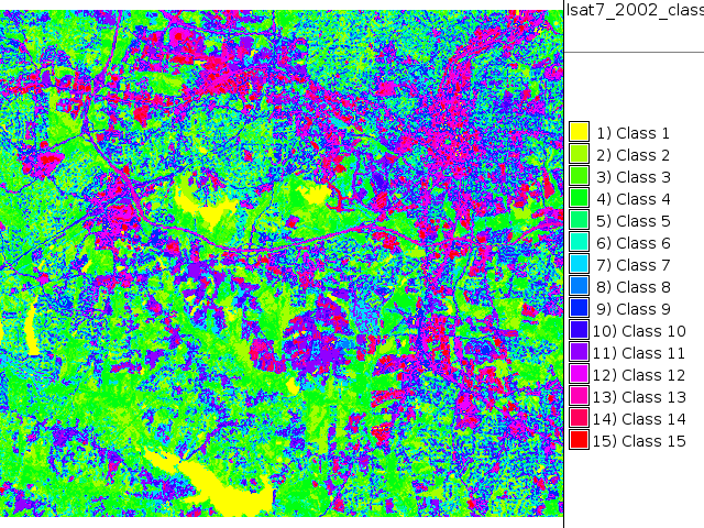
Supervised classification
Launch GUI for digitizer:
g.gui wxpython
Now digitize training areas of water, asphalt, forest, uncovered soil on RGB composite in GUI. Digitize polygons/centroids with attributes. The advantage: we know what the classes are.
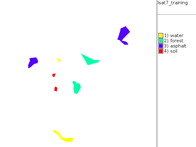
Assign also numerical ID for each class in new column
 v.db.select lsat7_training
 v.db.addcol lsat7_training col="id integer"
 v.db.select lsat7_training
 v.db.update lsat7_training col=id where="name = 'water'" val=1
 v.db.update lsat7_training col=id where="name = 'forest'" val=2
 v.db.update lsat7_training col=id where="name = 'asphalt'" val=3
 v.db.update lsat7_training col=id where="name = 'soil'" val=4
 v.db.select lsat7_training
Transform vector training map to raster model:
 g.region vect=lsat7_training align=lsat7_2002_10 -p
 v.to.rast in=lsat7_training out=lsat7_training use=attr col=id labelcol=name --o

 d.mon x0
 d.rast.leg lsat7_training
Generate statistics from training areas
i.gensigset group=lsat7_2002 subgroup=lsat7_2002 sig=lsat7_2002_smap training=lsat7_training
Perform supervised classification
i.smap group=lsat7_2002 subgroup=lsat7_2002 sig=lsat7_2002_smap out=smap
Colorize:
r.colors smap rules=- << EOF
1 aqua
2 green
3 180 180 180
4 brown
EOF
 d.rast.leg smap
 d.rgb b=lsat7_2002_10 g=lsat7_2002_20 r=lsat7_2002_30
 |
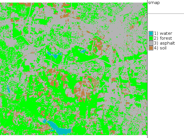 |
Vectorize result:
 r.to.vect smap out=smap feat=area
 d.rgb b=lsat7_2002_10 g=lsat7_2002_20 r=lsat7_2002_30
 d.vect smap  type=boundary col=red
That's it :)
Assessing the quality and result of the classification
- r.cross
- r.kappa
- r.change.info: Landscape change assessment
Further reading on classification with GRASS GIS
- Georganos, S., Lennert, M., Grippa, T., Vanhuysse, S., Johnson, B., Wolff, E., 2018. Normalization in Unsupervised Segmentation Parameter Optimization: A Solution Based on Local Regression Trend Analysis. Remote Sensing 10, 222. https://doi.org/10.3390/rs10020222
- Grippa, T., Lennert, M., Beaumont, B., Vanhuysse, S., Stephenne, N., Wolff, E., 2017. An Open-Source Semi-Automated Processing Chain for Urban Object-Based Classification. Remote Sensing 9, 358. https://doi.org/10.3390/rs9040358
- Beaumont, B., Grippa, T., Lennert, M., Vanhuysse, S.G., Stephenne, N.R., Wolff, E., 2017. Toward an operational framework for fine-scale urban land-cover mapping in Wallonia using submeter remote sensing and ancillary vector data. JARS, JARSC4 11, 036011. https://doi.org/10.1117/1.JRS.11.036011
- Micha Silver: Analyzing acacia tree health in the Arava with GRASS GIS
- Perrygeo: Impervious surface deliniation with GRASS
- Dylan Beaudette: Working with Landsat Data
- Dylan Beaudette: Canopy Quantification via Image Classification
- Segmentazione o classificazione d'immagini con GRASS (in italiano)
- Di Palma, F.; Amato, F.; Nolè, G.; Martellozzo, F.; Murgante, B. 2016: A SMAP Supervised Classification of Landsat Images for Urban Sprawl Evaluation. ISPRS Int. J. Geo-Inf. 2016, 5, 109. PDF: http://www.mdpi.com/2220-9964/5/7/109
Further reading on OBIA with GRASS GIS
- A complete toolchain for object-based image analysis with GRASS GIS