MB-System

• go to the Marine Science wiki page
• go to the GRASS and GMT wiki page

MB-System

• MB-System is Free software for the processing and display of swath and sidescan sonar data. It can handle both multibeam bathymetry and sidescan sonar image data.

Import into GRASS

• Gridded data can be loaded into GRASS either as a GMT NetCDF grid via the r.in.gdal module (see GDAL supported formats), old-style GMT grid using r.in.bin -h, or as an Arc ASCII grid via the r.in.arc module.

See the GRASS and GMT wiki help page for more information.

• Ungridded data points may be piped directly from mblist to GRASS's v.in.ascii module.

d.vect's zcolor= option can be used to color by 3D depth value.

Use the v.colors module for colorizing point data in GRASS (v.colors may be unsuitable for massive datasets).

• ".fnv" navigation files can be imported with the v.in.mbsys_fnv addon module in a number of different ways:

1. track: ship's track
2. port_trk: port-side outward track
3. stbd_trk: starboard-side outward track
4. scanlines: lines perpendicular to direction of travel
5. swath: coverage area
6. track_pts: ship's track as points
7. all_pts: ship's track, port, and stbd track points

Examples

Import x,y,z bathymetry into GRASS

Into a vector points map

• Export Lat/Lon + depth data from XTF datafile into a GRASS Lat/Lon location

 mblist -I 074.XTF -OXYz | v.in.ascii out=track074 x=1 y=2 fs=tab

• Export Lat/Lon from the XTF datafile, reproject into the current GRASS location's projection with m.proj, and import into GRASS with v.in.ascii

 mblist -I 074.XTF -OXY | m.proj -i | cut -f1 -d' ' | \
    v.in.ascii out=track074 x=1 y=2 fs=tab

* Idea: write a v.in.cdl script that will parse a NetCDF/CDL file and automatically set v.in.ascii's column= option with attribute table column names and SQL column types (INTEGER, FLOAT, VARCHAR(), DATE, etc.).

• Interpolate into a DEM with (for example) the v.surf.rst or the v.to.rast+r.surf.nnbathy modules.

Into a gridded raster map

• Read a series of .fbt pre-processed bathymetry files, reproject into the current projection (e.g. a local Transverse Mercator), and grid into raster maps.

First create .fbt .fnv and .inf summary files

 find . | grep '.[xX][tT][fF]$' > tmplist
 mbdatalist -F-1 -I tmplist > datalist-1 
 mbdatalist -F-1 -I datalist-1 -N

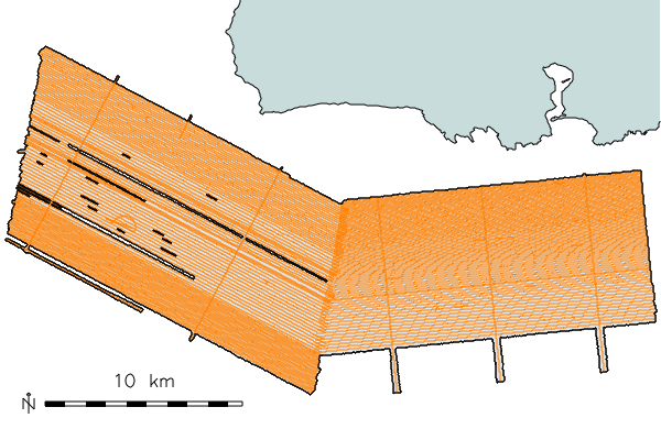
Next create quick GMT plot of the nav lines to check coverage

 # scan multi-dir for bounds
 for lltype in Longitude Latitude ; do
   for tb in head tail ; do
     grep $lltype `find | grep '\.inf$'` | \
       awk '{print $3 "\n" $6}' | sort -n | $tb -n1
   done
 done
 EXTENT=167.68/169.09/40.48/40.82
 
 mbdatalist -F-1 -I datalist-1 -R$EXTENT > survey-datalist
 mbm_plot -F-1 -I survey-datalist -N
 ./survey-datalist.cmd
 ps2ps survey-datalist.ps

Based on the above PostScript file set GRASS region by eye:

 LL: n=40:48N s=40:37N w=168:40E e=169:06E

Convert to local projection with m.proj:

 echo "168d40E 40d37N
 169d06E 40d48N" | m.proj -i

Plug those numbers into g.region:

 g.region s=4616845.02 n=4636836.33 w=520872.47 e=524862.14

Set the grid cell size to 5m, and align to whole numbers, and check that the rows x columns is reasonable (smaller than 40000x40000):

 g.region res=5 -a -p

Adjust resolution to smaller grid size if needed (1000x1000 rows,cols is fine for a summary image).

 g.region res=10 -a -p

Scan, read, and reproject all .fbt data into a single x,y,z text file:

A datalist fed to mblist then piped through 'm.proj -i' and r.in.xyz to form a gridded DEM.

Note that this file can get very large, perhaps too large for a 32bit OS/filesystem. In these cases you can pipe directly into r.in.xyz so no file is written to disk.

note that -Rw/e/s/n is used to skip over out-of-region data. MB-System and GMT will accept DDD:MM:SS.SSSh format as well as decimal degrees, just like GRASS.

The following assumes the output is projected, for import into WGS84 lat/lon skip the cs2cs command or at least change "%.3f" to "%.8f".

OUTPROJ="`g.proj -jf`"
( 
  for FILE in `find . | grep '\.fbt$'` ; do
    echo "Reading <$FILE> ..." 1>&2
    mblist -I$FILE -D3 -R168:40E/169:06E/40:37N/40:48N
  done 
) | cs2cs -f '%.3f' +init=epsg:4326 +to $OUTPROJ | \
   tr ' ' '\t' > fbt_UTM58_zoom.dat

Based on scan of the .inf files and personal knowledge set some reasonable bounds for the z-data:

# scan multi-dir for depth bounds
for tb in head tail ; do
   grep Depth `find | grep '\.inf$'` | \
      awk '{print $3 "\n" $6}' | sort -n | $tb -n1
done
#-2.7339
#200.6072

ZRANGE="-250,-2"

Run r.in.xyz to make aggregate raster maps.

r.in.xyz fs=tab x=1 x=2 z=3 zrange=$ZRANGE \
  in=zoom_fbt.dat out=zoom_fbt.n method=n

r.in.xyz fs=tab x=1 x=2 z=3 zrange=$ZRANGE \
  in=zoom_fbt.dat out=zoom_fbt.mean method=mean

r.in.xyz fs=tab x=1 x=2 z=3 zrange=$ZRANGE percent=25 \
  in=zoom_fbt.dat out=zoom_fbt.median method=median

r.in.xyz fs=tab x=1 x=2 z=3 zrange=$ZRANGE percent=25 \
  in=zoom_fbt.dat out=zoom_fbt.trim20 method=trimmean trim=20

Analyze "n" map for number of pings per square-meter.

no-data cells not randomly distributed so we set n=0 to NULL so we aren't biasing the data as much

 r.null zoom_fbt.n setnull=0
 r.univar zoom_fbt.n

"mean:" is number of pings per square-meter for cells which have data.

Now analyze bathymetry data:

 r.univar zoom_fbt.median

and set some nice colors:

 r.colors zoom_fbt.median color=bcyr

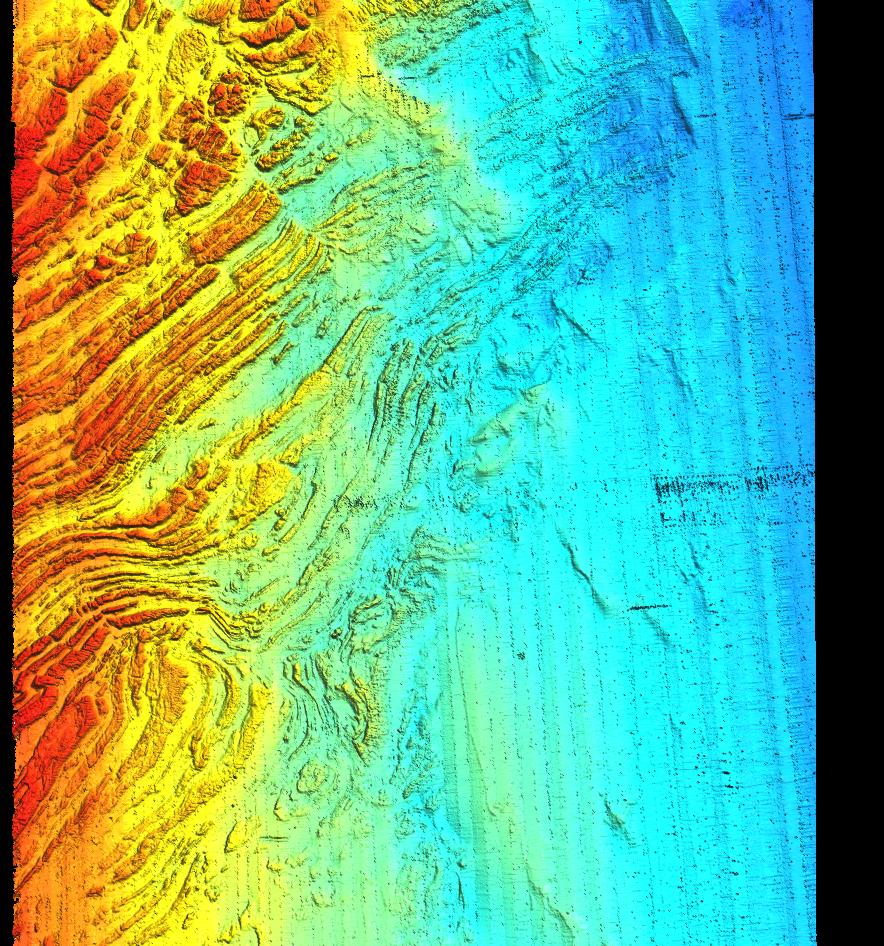
Finally display it:

 d.mon x0
 d.rast zoom_fbt.median
 d.legend zoom_fbt.median
 d.barscale at=5,5

Create vector maps from .fnv nav data

Add bounding box

MAP=swath_MBM04_007_0501_XTF

v.db.addcol $MAP column="north DOUBLE PRECISION, \
  south DOUBLE PRECISION, east DOUBLE PRECISION, west DOUBLE PRECISION"

eval `v.info -g $MAP`

echo "UPDATE $MAP SET north = $north, south = $south, \
  east = $east, west = $west" | db.execute

Import loop and patching

change DB to sqlite

db.connect driver=sqlite database='$GISDBASE/$LOCATION_NAME/$MAPSET/sqlite.db'

Import all files in the datalist using a loop:

for TYPE in track swath ; do
   for TRACK in `cut -f1 -d' ' datalist-1` ; do
      OUTNAME="${TYPE}_$( echo "`basename $TRACK .fnv`" | sed -e 's/[- .]/_/g' )"
      echo "Importing <$OUTNAME> ..."
 
      CAT=`echo "$OUTNAME" | cut -f3,4 -d'_' | tr -d '_'`
 
      v.in.mbsys_fnv in="${TRACK}.fnv" out="$OUTNAME" type=$TYPE cat=$CAT
   done
done

Patch together all maps with a loop:

for TYPE in track swath ; do

   # create an empty vector
   v.in.ascii -e out="datalist_${TYPE}s" --quiet

   # copy table structure
   BASE_MAP=`g.mlist vect pattern="${TYPE}_*" | head -n 1`
   exist_cols=`db.describe $BASE_MAP -c | grep '^Column' | cut -f2- -d: | \
     sed -e 's/:/ /' -e 's/CHARACTER:\(.*\)/VARCHAR(\1)/' | \
     cut -f1 -d: | tr '\n' ',' | sed -e 's/,$//' -e 's/^ //'`
   v.db.addtable "datalist_${TYPE}s" columns="$exist_cols"

   # run the patch loop
   for MAP in `g.mlist vect pattern="${TYPE}_*"` ; do
      echo "Patching <$MAP> ..."

      v.patch -a -e in="$MAP" out=datalist_${TYPE}s --overwrite --quiet

   done
done

• trac #859: v.patch is failing to preserve our carefully selected category numbers.

View and interactive query:

d.mon start=x0
d.vect datalist_swaths type=area color=150:170:200 fcolor=200:220:250
d.vect datalist_tracks width=2

d.zoom

d.what.vect datalist_tracks -f

Create a single coverage area

Convert all-swath patch into a single polygon:

(fast & good enough method)

This method generalizes the data by converting into a raster grid then back into a vector area.

# display and set region & raster resolution
d.vect datalist_swaths type=area fcolor=none
d.zoom
g.region -a -p res=

# initialize base map
r.mapcalc "swath_coverage = 0"

# loop to systematically add a "1" every time a cell is
#   covered by a swath; highlights overlap areas.
for MAP in `g.mlist vect pattern="swath_*"` ; do
   echo "Adding <$MAP> ..."
   v.to.rast in="$MAP" use=val val=1 type=area out=tmp.$MAP.$$ --quiet
   r.series in=swath_coverage,tmp.$MAP.$$ method=sum out=tmp.series.$$ --quiet
   g.remove tmp.$MAP.$$,swath_coverage --quiet
   g.rename tmp.series.$$,swath_coverage --quiet
done

# flatten to a boolean coverage mask map
r.reclass in=swath_coverage out=swath_coverage.1 << EOF
  1 thru 999999 = 1
  0 = NULL
EOF

# convert back to a vector area polygon
r.to.vect -s -v in=swath_coverage.1 out=Swath_coverage feature=area

# remove tiny holes (single or a few cells)
v.clean in=Swath_coverage out=Swath_coverage_noHoles tool=rmarea thresh=10000

Survey swaths imported with v.in.mbsys_fnv and combined into a single coverage area. Track lines are overlain.

Clean all-swath patch into a single polygon:

(much slower but more exact method)

v.db.addcol map=datalist_swaths column='cat1 integer'
v.db.update map=datalist_swaths column=cat1 value=1
v.reclass in=datalist_swaths out=swaths1 column=cat1
v.db.dropcol map=datalist_swaths column=cat1 
# this cleaning step may take a ''very'' long time
v.clean tool=break in=swaths1 out=swaths2
v.dissolve in=swaths2 out=datalist_swaths_coverage
g.remove vect=swaths1,swaths3

Export to GMT

Processed raster grids and vector areas, lines, and points can be exported to back to GMT for plotting. See the GRASS and GMT wiki page for more information.