Image processing/Evapotranspiration: Difference between revisions
m (→See also) |
m (→Introduction) |
||
| Line 4: | Line 4: | ||
Atmospheric transfer of '''irradiance''' is subject to atmosphere particles interactions, scattering, diffraction, reflection, etc. | Atmospheric transfer of '''irradiance''' is subject to atmosphere particles interactions, scattering, diffraction, reflection, etc. | ||
When reaching the planetary surface, is it partially reflected in the shortwave by '''Albedo'''. Surface Albedo is the integrated 0.3-3 micro-meters reflectance, it reflects the shortwave energy coming from the sun by 5% on oceans, 15-25% on vegetation, 35-40% on sand/desert/beach, 60-80% on snow/clouds, roughly. This energy fraction is returned to atmosphere for complex interaction with gas particles again before leaving the atmosphere altogether. | When reaching the planetary surface, is it partially reflected in the shortwave by '''Albedo'''. | ||
Surface Albedo is the integrated 0.3-3 micro-meters reflectance, it reflects the shortwave energy coming from the sun by 5% on oceans, 15-25% on vegetation, 35-40% on sand/desert/beach, 60-80% on snow/clouds, roughly. This energy fraction is returned to atmosphere for complex interaction with gas particles again before leaving the atmosphere altogether. | |||
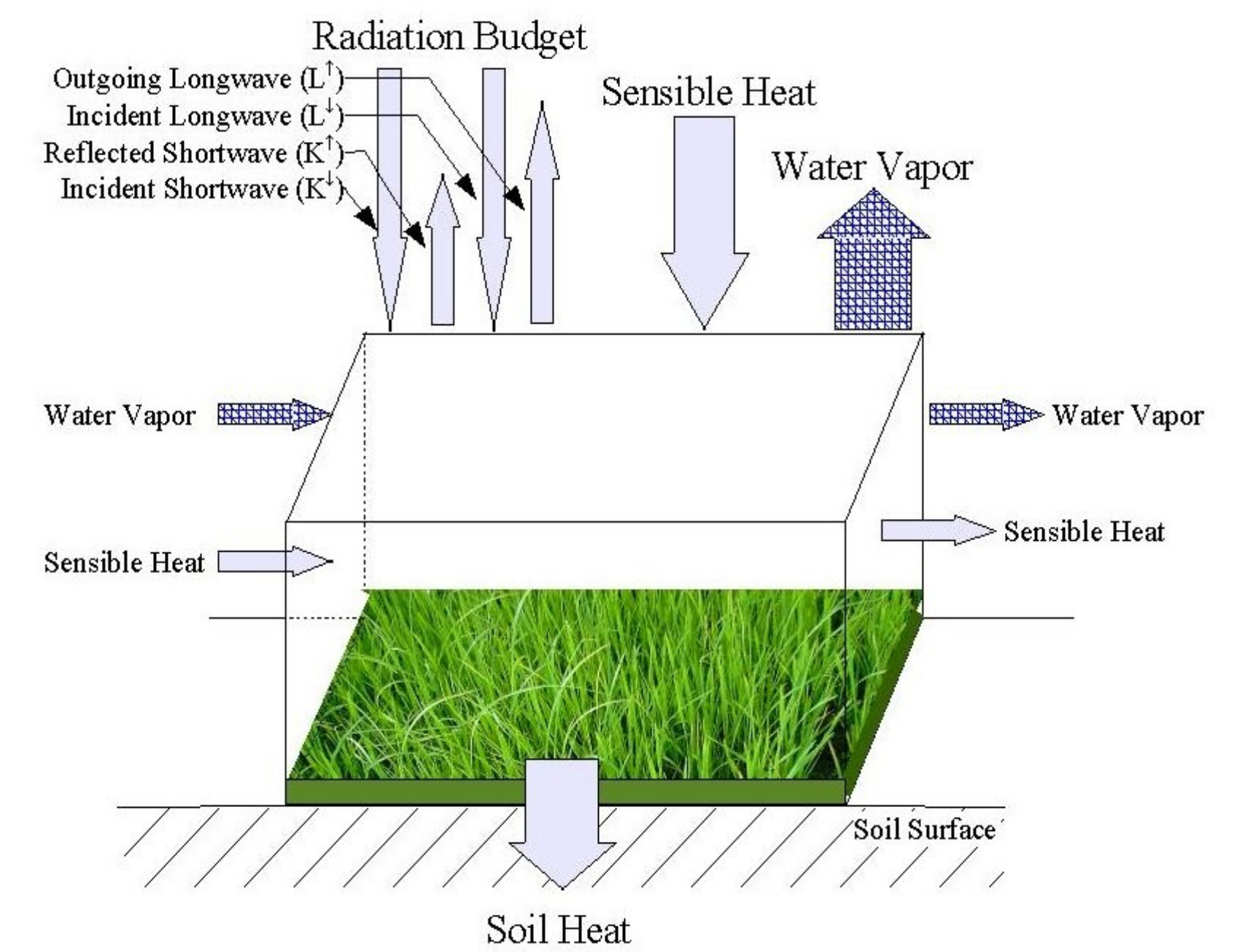
[[File:EnergyBalance.png||500px||Alt="Chemin, 2006, PhD Thesis"]] | [[File:EnergyBalance.png||500px||Alt="Chemin, 2006, PhD Thesis"]] | ||
As for the shortwave surface balance, the '''energy''' is also received in the longwave, but interacts with the grey-body characteristics of the surface elements. The blackbody to greybody fraction is ruled by emissivity, a hidden component in the thermal spectrum (search for Temperature- Emissivity Separation algorithms). On Earth, emissivity is always above 0.9 (mostly 0.96-0.98). The Stefan-Boltzman equation is dealing with blackbody energy, and multiplying it by Emissivity transforms it to greybody energy emitted. | As for the shortwave surface balance, the '''energy''' is also received in the longwave, but interacts with the grey-body characteristics of the surface elements. | ||
The blackbody to greybody fraction is ruled by emissivity, a hidden component in the thermal spectrum (search for Temperature- Emissivity Separation algorithms). On Earth, emissivity is always above 0.9 (mostly 0.96-0.98). The Stefan-Boltzman equation is dealing with blackbody energy, and multiplying it by Emissivity transforms it to greybody energy emitted. | |||
Together, shortwave and longwave '''energy balance''' provide with the net radiation balance at the surface of the planetary body. This crucial term is the total energy available for thermodynamic fluxes to act on the surface of the planet. | |||
On a planet like Earth where there is a triple phase of a given molecule (H20, in gas, liquid, solid), energy available is used to transfer phases from lower energy to higher energy (sublimation, liquefaction, evaporation). Thermal transfers also happen as conduction (soil, rocks) and convection (atmosphere, oceans). | |||
The i.eb.* modules and models deal with: | The i.eb.* modules and models deal with: | ||
Revision as of 08:26, 2 December 2023
Introduction
The radiation is coming from the planet's star, Earth has around 1800 W/m2 of incoming radiation from the sun (also called irradiance) at exo-atmospheric altitude.
Atmospheric transfer of irradiance is subject to atmosphere particles interactions, scattering, diffraction, reflection, etc.
When reaching the planetary surface, is it partially reflected in the shortwave by Albedo.
Surface Albedo is the integrated 0.3-3 micro-meters reflectance, it reflects the shortwave energy coming from the sun by 5% on oceans, 15-25% on vegetation, 35-40% on sand/desert/beach, 60-80% on snow/clouds, roughly. This energy fraction is returned to atmosphere for complex interaction with gas particles again before leaving the atmosphere altogether.
As for the shortwave surface balance, the energy is also received in the longwave, but interacts with the grey-body characteristics of the surface elements.
The blackbody to greybody fraction is ruled by emissivity, a hidden component in the thermal spectrum (search for Temperature- Emissivity Separation algorithms). On Earth, emissivity is always above 0.9 (mostly 0.96-0.98). The Stefan-Boltzman equation is dealing with blackbody energy, and multiplying it by Emissivity transforms it to greybody energy emitted.
Together, shortwave and longwave energy balance provide with the net radiation balance at the surface of the planetary body. This crucial term is the total energy available for thermodynamic fluxes to act on the surface of the planet.
On a planet like Earth where there is a triple phase of a given molecule (H20, in gas, liquid, solid), energy available is used to transfer phases from lower energy to higher energy (sublimation, liquefaction, evaporation). Thermal transfers also happen as conduction (soil, rocks) and convection (atmosphere, oceans).
The i.eb.* modules and models deal with:
- conduction i.eb.soilheatflux (for thermal conduction in soils)
- convection i.eb.h_* especially (for thermal convection in atmosphere)
- residual method estimating the energy left for evaporation processes (i.eb.evapfr, i.eb.eta are examples).
Additionally, a helper module i.eb.z0m is producing an estimation of the surface roughness, necessary in latent heat flux estimation.
i.evapo.* modules/models are integrated models
from the oldest that are not based on energy balance, but are computing some form of evapotranspiration (ETo: Evapotranspiration for a reference of 20cm well-watered grass, see FAO no56 report of Richard Allen)
- Penman-Monteith i.evapo.pm
- Priestley-Taylor i.evapo.pt
- Hargreaves i.evapo.mh
to newer that are in some form or another linked to thermal processes.
- Thermal index i.evapo.senay
- Biome thermal processes i.evapo.zk (global model based on typical info from biomes Albedo/soil heat flux)
- Thermodynamic processes i.evapo.potrad (potential ET if not water stress, based on astronomical equations only)
Most developed thermodynamic models are:
- TSEB (i.evapo.tseb: Two Source Energy Balance, Schmugge, Kustas, etc., 2000) Status: Incomplete Module
- SEBS (i.evapo.sebs: Zhu et al, 2002) Status: Incomplete Module
- SEBAL i.eb.h_sebal01, i.eb.evapfr, i.eb.eta (Bastiaanssen et al, 1998, 2001)
and some newer models like RESET and others. The list of models using thermodynamic principles is large now, and any willing to submit a code for any of them is most welcome.
Temporal Integration of Evapotranspiration
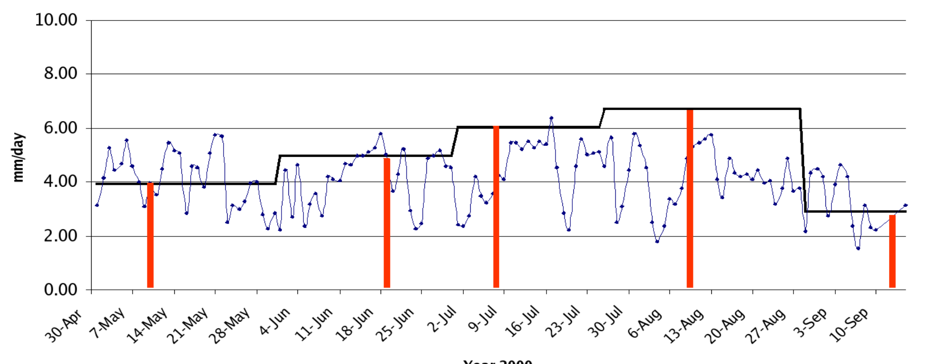
When integrated in time i.evapo.time, seasonal evapotranspiration can be computed and therefore permit a full monitoring of vegetation growth over the period. This is also a basis of crop yield estimation (see i.biomass).
See also
- Manual pages:
- Evapotranspiration mapping with Landsat 5TM in GRASS GIS
Example script to process Landsat 8 Evapotranspiration
#!/bin/bash

# This scripts imports, pre-processes and compute Evapotranspiration for Landsat 8
# Run in a Location compatible with your L8 dataset

# Atmospheric Transmissivity single-way
tsw=0.75
# Light Use Efficiency (please change dependent on your crop/plant)
lue=1.0

# Import files in GRASS
for file in *TIF
do
	r.in.gdal -e input=$file output=$(echo $file | sed 's/.TIF//') --o
done
# Set region to newly imported files
g.region -s raster=$(ls *TIF | grep B1.TIF | sed 's/.TIF//')
LC08=$(ls *TIF | grep B1.TIF | sed 's/1.TIF//')

# Set metadata MTL file name
LC08met=$(ls *MTL.txt)

# Import DEM
r.import input=dem.tif output=dem extent=region --o
# Extract date
date=$(i.landsat.toar input=$LC08 output=l8 metfile=$LC08met lsatmet=date --o)
echo $date

# Apply Top of Atmosphere correction
i.landsat.toar input=$LC08 output=l8 metfile=$LC08met --o

# Set NODATA
for file in $(g.list type=raster pattern=LC08*)
do
	r.null map=$file setnull=0
done

#Set computing area to B10 active pixels
for n in 1 2 3 4 5 6 7 8 9
do
	r.mapcalc expression="temp=if(isnull(l810),null(),l8$n)" --o
	g.rename raster=temp,l8$n --o
done

base=l8
# Create config files for 6s
year=$(cat *MTL* | grep DATE_ACQUIRED | grep -oP '(=)[^;]+' | sed 's/=\ \(.*\)/\1/' | sed 's/\(.*\)-\(.*\)-\(.*\)/\1/')
mm=$(cat *MTL* | grep DATE_ACQUIRED | grep -oP '(=)[^;]+' | sed 's/=\ \(.*\)/\1/' | sed 's/\(.*\)-\(.*\)-\(.*\)/\2/')
dd=$(cat *MTL* | grep DATE_ACQUIRED | grep -oP '(=)[^;]+' | sed 's/=\ \(.*\)/\1/' | sed 's/\(.*\)-\(.*\)-\(.*\)/\3/')
doy=$( date -I -d "$year-$mm-$dd" | date +%j)
hh=$(cat *MTL* | grep TIME | grep -oP '(=)[^;]+' | sed 's/=\ \"\(.*\):\(.*\):\(.*\)\.\(.*\)/\1/')
mn=$(cat *MTL* | grep TIME | grep -oP '(=)[^;]+' | sed 's/=\ \"\(.*\):\(.*\):\(.*\)\.\(.*\)/\2/')
ss=$(cat *MTL* | grep TIME | grep -oP '(=)[^;]+' | sed 's/=\ \"\(.*\):\(.*\):\(.*\)\.\(.*\)/\3/')
time=$(echo "$hh + ($mn / 60.0) + ($ss / 3600.0)" | bc -l)
lat=$(echo $(cat *MTL* | grep CORNER_ | grep LAT | grep -oP '(=)[^;]+' | sed 's/=//' | awk '{s+=$1} END {print s}') "/4.0" |  bc -l)
lon=$(echo $(cat *MTL* | grep CORNER_ | grep LON | grep -oP '(=)[^;]+' | sed 's/=//' | awk '{s+=$1} END {print s}') "/4.0" |  bc -l)
echo "18                            - geometrical conditions=Landsat 8" > 6s_conf.txt
echo "$mm $dd $hh.$mm $lon $lat    - month day hh.ddd longitude latitude ("hh.ddd" is in GMT decimal hours)" >> 6s_conf.txt
echo "1                            - atmospheric model=midlatitude summer" >> 6s_conf.txt
echo "1                            - aerosols model=continental" >> 6s_conf.txt
echo "24                           - visibility [km] (aerosol model concentration)" >> 6s_conf.txt
echo "-0.110                       - mean target elevation above sea level [km]" >> 6s_conf.txt
echo "-1000                        - sensor on board a satellite" >> 6s_conf.txt
#For Band 1:
cat 6s_conf.txt > $base\1_conf.txt
echo "115                           - Coastal band of OLI Landsat 8" >> $base\1_conf.txt
#For Band 2:
cat 6s_conf.txt > $base\2_conf.txt
echo "116                           - Blue band of OLI Landsat 8" >> $base\2_conf.txt
#For Band 3:
cat 6s_conf.txt > $base\3_conf.txt
echo "117                           - Green band of OLI Landsat 8" >> $base\3_conf.txt
#For Band 4:
cat 6s_conf.txt > $base\4_conf.txt
echo "118                           - Red band of OLI Landsat 8" >> $base\4_conf.txt
#For Band 5:
cat 6s_conf.txt > $base\5_conf.txt
echo "120                           - NIR band of OLI Landsat 8" >> $base\5_conf.txt
#For Band 6:
cat 6s_conf.txt > $base\6_conf.txt
echo "122                           - SWIR1 band of OLI Landsat 8" >> $base\6_conf.txt
#For Band 7:
cat 6s_conf.txt > $base\7_conf.txt
echo "123                           - SWIR2 band of OLI Landsat 8" >> $base\7_conf.txt
#For Band 8:
cat 6s_conf.txt > $base\8_conf.txt
echo "119                           - PAN band of OLI Landsat 8" >> $base\8_conf.txt
#For Band 9:
cat 6s_conf.txt > $base\9_conf.txt
echo "121                           - Cirrus band of OLI Landsat 8" >> $base\9_conf.txt

# Compute Atmospheric correction
for file in $base\1 $base\2 $base\3 $base\4 $base\5 $base\6 $base\7 $base\8 $base\9
do
	i.atcorr -r $file elevation=dem parameters=$file\_conf.txt output=s$file --o
	r.mapcalc expression="temp=if(isnull(l810),null(),s$file)" --o
	g.rename raster=temp,s$file --o
	r.colors map=$file color=grey
done

# Create cloud Mask
g.rename raster=l83,l7.2
g.rename raster=l84,l7.3
g.rename raster=l85,l7.4
g.rename raster=l86,l7.5
g.rename raster=l810,l7.6
i.landsat.acca -5 -f input=l7. output=temp --o
g.rename raster=l7.2,l83
g.rename raster=l7.3,l84
g.rename raster=l7.4,l85
g.rename raster=l7.5,l86
g.rename raster=l7.6,l810
r.mapcalc expression="temp1=if(isnull(temp),0,1)" --o
r.mapcalc expression="maskVIS=if(isnull(l810),null(),temp1)" --o

# Apply mask
r.mask raster=maskVIS maskcats=0

# Latitude map
r.latlong input=l81 output=latitude --o

# Longitude map
r.latlong -l input=l81 output=longitude --o

# i.albedo
i.albedo -8 -c input=sl81,sl82,sl83,sl84,sl85,sl86,sl87 output=l8alb --o
r.colors -e map=l8alb color=grey

# i.vi viname=ndvi
i.vi viname=ndvi red=sl84 nir=sl85 output=l8ndvi --o
r.colors map=l8ndvi color=ndvi

# Update processing mask with water
r.mapcalc expression="maskWATER=if(l8ndvi<=0,0,maskVIS)" --o
r.mask -r
r.mask raster=maskWATER maskcats=0

# i.emissivity
i.emissivity input=l8ndvi output=l8emis --o

# i.vi viname=savi
i.vi viname=savi red=sl84 nir=sl85 output=l8savi --o
r.colors map=l8savi color=ndvi

# Daily Net Radiation (RNETD)
r.mapcalc expression="temp=if(isnull(l810),null(),dem)" --o
r.slope.aspect elevation=temp slope=slopedd aspect=aspectdd --o
r.sun elevation=temp aspect=aspectdd slope=slopedd albedo=l8alb glob_rad=rnetd insol_time=sunhours day=$doy nprocs=8 --o
r.mapcalc expression="l8rnetd=rnetd/sunhours" --o

# Instantaneous Net Radiation (RNET)
timelocal=$(echo "$time + (24.0 / 360.0) * $lon" | bc -l)
r.sun elevation=temp aspect=aspectdd slope=slopedd albedo=l8alb glob_rad=l8rnet day=$doy time=$timelocal nprocs=8 --o

# Soil Heat Flux (G0)
r.mapcalc expression="overpasstime=$time" --o
i.eb.soilheatflux albedo=l8alb ndvi=l8ndvi temperature=l810 netradiation=l8rnet localutctime=overpasstime output=l8g0 --o

# Sensible Heat Flux (H)
i.eb.z0m -p input=l8savi output=z0m --o
r.mapcalc expression="T0dem=0.00612*dem+l810" --o
i.eb.hsebal01 -a netradiation=l8rnet soilheatflux=l8g0 aerodynresistance=z0m temperaturemeansealevel=T0dem frictionvelocitystar=0.32407 vapourpressureactual=1.511 output=l8h --o

# Evaporative Fraction & Soil Moisture
i.eb.evapfr -m netradiation=l8rnet soilheatflux=l8g0 sensibleheatflux=l8h evaporativefraction=l8evapfr soilmoisture=l8sm --o

# Actual Evapotranspiration (ETa)
i.eb.eta netradiationdiurnal=l8rnetd evaporativefraction=l8evapfr temperature=l810 output=l8eta --o

# Biomass growth
r.mapcalc expression="l8fpar=1.257*l8ndvi-0.161" --o
r.mapcalc expression="doy=$doy" --o
r.mapcalc expression="tsw=$tsw" --o
r.mapcalc expression="lue=$lue" --o
i.biomass fpar=l8fpar lightuse_efficiency=lue latitude=latitude dayofyear=doy transmissivity_singleway=tsw water_availability=l8evapfr output=l8biom --o

# Export everything we need
for rstF in l8eta l8sm l8biom l8ndvi l8alb l8rnet l8g0 l8rnetd
do
	r.null map=$rstF setnull=-100000-0
	r.out.gdal -c -m input=$rstF output=$rstF\_$year$mm$dd.tif nodata=-32768 --o
done

