R statistics: Difference between revisions
| Line 93: | Line 93: | ||
* Usage II (taken from the grass-stats-ML): | * Usage II (taken from the grass-stats-ML): | ||
http://lists.osgeo.org/pipermail/grass-stats/2010-September/001274.html | |||
at the moment there is following for a Grass-R-connection implemented in WinGrass64 | at the moment there is following for a Grass-R-connection implemented in WinGrass64 | ||
| Line 105: | Line 107: | ||
with this starting option you start a Grass-session in the good old text mode. | with this starting option you start a Grass-session in the good old text mode. | ||
if you type R in the command line, then you start R inside a Grass-session like in Linux. | if you type R in the command line, then you start R inside a Grass-session like in Linux. | ||
[...] | [...] | ||
Ticket #1103 (new enhancement) WinGrass64 - windows-commandline not released: | |||
a Grass-session with wxGui, command-line and R inside a Grass-session would | |||
be possible (as already does in WinGrass7) | be possible (as already does in WinGrass7) | ||
Ticket #1149 (new enhancement) WinGrass - load R-installation-path dynamically into PATH: | |||
Wingrass would recognize also an upgraded R-installation (which does not at the moment) | |||
=== Command help === | === Command help === | ||
Revision as of 21:38, 24 September 2010
Q: How do I enjoy high quality statistic analysis in GRASS?
A: Well, GRASS has got an interface to the most powerful statistics analysis package around: R (http://www.r-project.org)
- The spgrass6 R addon package provides the R ←→ GRASS interface.
Quick start
For the impatient just start it:
 > R

 #and install packages directly from the net
 pkgs <- c('akima', 'spgrass6', 'RODBC', 'VR', 'gstat')

 install.packages(pkgs, dependencies=TRUE, type='source')
Once you have R and spgrass6 on your system, have a look at this tutorial:
Installation
First of all you need to install R onto your system.
R and many of its addon packages are pre-built and distributed through the CRAN network of mirrors. In addition many Linux distributions prepackage R and a number of the most popular addon toolboxes.
All the necessary functions for the GRASS 6 interface are now in packages on CRAN, so that on Linux/Unix (or Mac OSX) installing rgdal from source with PROJ4 and GDAL installed, or Windows installing from binary, the required packages are: sp; maptools (now includes spmaptools); rgdal (now includes spGDAL, spproj); spgrass6 - now all on CRAN.
Source packages
From the R console first pick a local mirror:
chooseCRANmirror()
you can then see what it picked with
options("repos")
To permanently save the mirror site add it to ~/.Rprofile. For example:
options(repos=c(CRAN="http://cran.stat.auckland.ac.nz"))
and then run install.packages() as in the Quick Start section above.
For more information see http://cran.r-project.org/doc/manuals/R-admin.html
Linux
Debian and Ubuntu
R and a number of pre-build cran packages are already present in the main repositories. Start with:
# apt-get install r-base r-cran-vr r-cran-rodbc r-cran-xml
Once those are installed start "R" at the command prompt and install the libraries not packaged by the OS:
install.packages("sp")
install.packages("gstat")
Debian/Lenny ships with R 2.7.1 which is too old for the modern rgdal package. So we have to fetch an old one from the archive and build it from the Linux command line:
$ wget http://cran.r-project.org/src/contrib/Archive/rgdal/rgdal_0.6-24.tar.gz
$ R CMD INSTALL -l /usr/local/lib/R/site-library rgdal_0.6-24.tar.gz
And finally, back inside the R session:
install.packages("spgrass6")
You can also use the CRAN Debian package repository: (pick one; adjust distribution as needed [here "Debian/testing"])
deb http://debian.cran.r-project.org/cran2deb/debian-i386 testing/
deb http://debian.cran.r-project.org/cran2deb/debian-amd64 testing/
RPM based
- RedHat, Suse, Mandrake and similar distros: take the latest R RPM and install it
Mac OSX
- for install.packages() you might have to rely on building packages from source code. try:
install.packages("spgrass6", type="source", dependencies = TRUE)
MS Windows
- Installation:
install.packages("spgrass6", dependencies = TRUE)
- Usage I:
On Windows, the easiest way is calling GRASS from R with initGRASS() from the R package spgrass6. After GRASS has been initialized for R, you have access to GRASS commands from within R. For an example, see http://geomorphometry.org/content/geomorphometry-r-saga-ilwis-grass
Go down to the part of the script with the GRASS example, adjust
loc <- initGRASS("C:/GRASS", home=tempdir())
as appropriate for your system.
- Usage II (taken from the grass-stats-ML):
http://lists.osgeo.org/pipermail/grass-stats/2010-September/001274.html
at the moment there is following for a Grass-R-connection implemented in WinGrass64
(1) the WinGrass64-installer searches during installation for a installed R and writes - if found - the R-installation-path to %PATH% in the grass64.bat-starting script (see http://trac.osgeo.org/grass/browser/grass/branches/develbranch_6/mswindows/GRASS-Installer.nsi#L660)
(2) you can start "Grass-command-line" - it's a windows-command-line, not a msys-rxvt-terminal (you can find this starting option under Programs -> Grass64 -> Grass command line; but not as a desktop icon)
with this starting option you start a Grass-session in the good old text mode. if you type R in the command line, then you start R inside a Grass-session like in Linux.
[...]
Ticket #1103 (new enhancement) WinGrass64 - windows-commandline not released:
a Grass-session with wxGui, command-line and R inside a Grass-session would be possible (as already does in WinGrass7)
Ticket #1149 (new enhancement) WinGrass - load R-installation-path dynamically into PATH:
Wingrass would recognize also an upgraded R-installation (which does not at the moment)
Command help
Start the R help browser:
help.start()
- Select Packages and then spgrass6.
Running
- by Roger Bivand
The R interface for GRASS 5.4 was provided by a CRAN package called grass. Changes going forward to the current GRASS 6 release meant that the interface had to be rewritten, and this provided the opportunity to adapt it to the sp CRAN package classes. Because GRASS provides the same kinds of data as sp classes handle, and relies on much of the same open source infrastructure (PROJ.4, GDAL, OGR), this step seemed sensible. Wherever possible spgrass6 tries to respect the current region in GRASS to avoid handling raster data with different resolutions or extents. R is assumed to be running within GRASS:
Startup
- Start GRASS. At the GRASS command line start R.
- In this example we will use the sample Spearfish dataset.
Reset the region settings to the defaults
GRASS> g.region -d
Load the spgrass6 library:
> library(spgrass6)
Get the GRASS environment (mapset, region, map projection, etc.)
> G <- gmeta6()
Reading in data
Read in two raster maps:
> spear <- readRAST6(c("geology", "elevation.dem"),
+          cat=c(TRUE, FALSE), ignore.stderr=TRUE,
+          plugin=NULL)
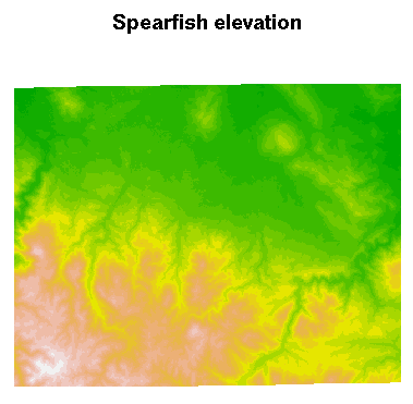
The metadata are accessed and available, but are not (yet) used to structure the sp class objects, here a SpatialGridDataFrame object filled with data from two Spearfish layers. Here is a plot of the elevation data:
> image(spear, attr = 2, col = terrain.colors(20))
Add a title to the plot:
> title("Spearfish elevation")

In addition, we can show what is going on inside the objects read into R:
> str(G)
List of 26
 $ GISDBASE     : chr "/home/rsb/topics/grassdata"
 $ LOCATION_NAME: chr "spearfish57"
 $ MAPSET       : chr "rsb"
 $ DEBUG        : chr "0"
 $ GRASS_GUI    : chr "text"
 $ projection   : chr "1 (UTM)"
 $ zone         : chr "13"
 $ datum        : chr "nad27"
 $ ellipsoid    : chr "clark66"
 $ north        : num 4928010
 $ south        : num 4913700
 $ west         : num 589980
 $ east         : num 609000
 $ top          : num 1
 $ bottom       : num 0
 $ nsres        : num 30
 $ nsres3       : num 30
 $ ewres        : num 30
 $ ewres3       : num 30
 $ tbres        : num 1
 $ rows         : int 477
 $ rows3        : int 477
 $ cols         : int 634
 $ cols3        : int 634
 $ depths       : int 1
 $ proj4        : chr "+proj=utm +zone=13 +a=6378206.4 +rf=294.9786982 +no_defs +nadgrids=/home/rsb/topics/grass61/grass-6.1.cvs/etc/nad/conus"
> summary(spear)
Object of class SpatialGridDataFrame
Coordinates:
              min     max
coords.x1  589980  609000
coords.x2 4913700 4928010
Is projected: TRUE
proj4string : [+proj=utm +zone=13 +a=6378206.4 +rf=294.9786982 +no_defs +nadgrids=/home/rsb/topics/grass61/grass-6.1.cvs/etc/nad/conus]
Number of points: 2
Grid attributes:
  cellcentre.offset cellsize cells.dim
1            589995       30       634
2           4913715       30       477
Data attributes:
      geology      elevation.dem
 sandstone:74959   Min.   : 1066
 limestone:61355   1st Qu.: 1200
 shale    :46423   Median : 1316
 sand     :36561   Mean   : 1354
 igneous  :36534   3rd Qu.: 1488
 (Other)  :37636   Max.   : 1840
 NA's     : 8950   NA's   :10101
Summarizing data
We can create a table of cell counts:
> table(spear$geology)
| metamorphic | transition | igneous | sandstone | limestone | shale | sandy shale | claysand | sand |
|---|---|---|---|---|---|---|---|---|
| 11693 | 142 | 36534 | 74959 | 61355 | 46423 | 11266 | 14535 | 36561 |
And compare with the equivalent GRASS module:
- FIXME: is system() still the recommended method?
> system("r.stats -cl geology")
1 metamorphic 11693
2 transition 142
3 igneous 36534
4 sandstone 74959
5 limestone 61355
6 shale 46423
7 sandy shale 11266
8 claysand 14535
9 sand 36561
* no data 8950
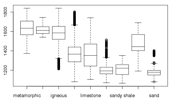
Create a box plot of geologic types at different elevations:
> boxplot(spear$elevation.dem ~ spear$geology, medlwd = 1)

Exporting data back to GRASS
Finally, a SpatialGridDataFrame object is written back to a GRASS raster map:
First prepare some data: (square root of elevation)
> spear$sqdem <- sqrt(spear$elevation.dem)
Export data from R back into a GRASS raster map:
> writeRAST6(spear, "sqdemSP", zcol="sqdem", ignore.stderr=TRUE)
Check that it imported into GRASS ok:
> system("r.info sqdemSP")
 +----------------------------------------------------------------------------+
 | Layer:    sqdemSP                        Date: Sun May 14 21:59:26 2006    |
 | Mapset:   rsb                            Login of Creator: rsb             |
 | Location: spearfish57                                                      |
 | DataBase: /home/rsb/topics/grassdata                                       |
 | Title:     ( sqdemSP )                                                     |
 |----------------------------------------------------------------------------|
 |                                                                            |
 |   Type of Map:  raster              Number of Categories: 255              |
 |   Data Type:    FCELL                                                      |
 |   Rows:         477                                                        |
 |   Columns:      634                                                        |
 |   Total Cells:  302418                                                     |
 |        Projection: UTM (zone 13)                                           |
 |            N:    4928010    S:    4913700   Res:    30                     |
 |            E:     609000    W:     589980   Res:    30                     |
 |   Range of data:    min =  32.649654 max = 42.895222                       |
 |                                                                            |
 |   Data Source:                                                             |
 |                                                                            |
 |                                                                            |
 |                                                                            |
 |   Data Description:                                                        |
 |    generated by r.in.gdal                                                  |
 |                                                                            |
 |                                                                            |
 +----------------------------------------------------------------------------+
Getting Support
- Primary support for R + GRASS and the spgrass6 package is through the grass-stats mailing list.
GRASS Modules
- v.krige: Perform kriging operations in the GRASS environment, using R software functions in background.
- Special requirements: python-rpy2 (not python-rpy!)
(merge info from man page here)
See also
- R. Bivand, 2007: Interfacing R and OSGeo projects: status and perspectives (Presentation with slides and scripts)
- Using GRASS and R: http://grass.osgeo.org/statsgrass/grass6_r_interface.html
- Connecting R to RDBMS: http://grass.osgeo.org/statsgrass/r_and_dbms.html
- Neural Networks with GRASS and R (posted by Markus Neteler on the grass-user mailing list) http://www.uam.es/proyectosinv/Mclim/pdf/MBenito_EcoMod.pdf
- A detailed example on the use of GRASS and R, with spearfish data: http://casoilresource.lawr.ucdavis.edu/drupal/node/438
- Using R and GRASS with cygwin: It is possible to use Rterm inside the GRASS shell in cygwin, just as in Unix/Linux or OSX. You should not, however, start Rterm from a cygwin xterm, because Rterm is not expecting to be run in an xterm under Windows, and loses its input. If you use the regular cygwin bash shell, but need to start display windows, start X from within GRASS with startx &, and then start Rterm in the same cygwin shell, not in the xterm.
- Spatial data in R (
sp) is a R library that provides classes and methods for spatial data (points, lines, polygons, grids), and to new or existing spatial statistics R packages that use sp, depend on sp, or will become dependent onsp, such asmaptools,rgdal,splancs,spgrass6,gstat,spgwrand many others.
- RPy - Python interface to the R Programming Language
Articles
- GRASS News vol.3, June 2005 (R. Bivand. Interfacing GRASS 6 and R. GRASS Newsletter, 3:11-16, June 2005. ISSN 1614-8746).
- OSGeo Journal vol. 1 May 2007 (R. Bivand. Using the R— GRASS interface. OSGeo Journal, 1:31-33, May 2007. ISSN 1614-8746).
- GRASS Book, last chapter