R statistics/rgrass: Difference between revisions
Veroandreo (talk | contribs) (rewrite to rgrass7 and North Carolina sample dataset) |
Veroandreo (talk | contribs) No edit summary |
||
| Line 1: | Line 1: | ||
'''This page refers to the usage of R within a GRASS GIS 7 session.''' (see also [[R_statistics/spgrass6]]) | '''This page refers to the usage of R within a GRASS GIS 7 session and the use of GRASS GIS 7 within an R session.''' (see also [[R_statistics/spgrass6]]) | ||
== R within GRASS == | |||
=== Startup === | === Startup === | ||
| Line 219: | Line 221: | ||
| | | | | | ||
| Comments: | | | Comments: | | ||
| | | | | | ||
+----------------------------------------------------------------------------+ | +----------------------------------------------------------------------------+ | ||
</pre> | </pre> | ||
=== Calling RStudio from a GRASS GIS session === | |||
If you are most used to run R through RStudio, but still want to have all GRASS data available for performing | |||
any analyses without loosing the possibility of still using GRASS command line, you can run: | |||
<pre> | |||
GRASS> rstudio & | |||
</pre> | |||
or, if you already are working on a certain RStudio project: | |||
<pre> | |||
GRASS> rstudio /path/to/project/folder/ & | |||
</pre> | |||
Then, you load rgrass7 library in your RStudio project | |||
> library(rgrass7) | |||
and you are ready to go. | |||
== GRASS within R == | |||
To call GRASS GIS 7 functionality from R, use the initGRASS() function to define the GRASS settings: | |||
<pre> | |||
library(rgrass7) | |||
# initialisation and the use of North Carolina sample dataset | |||
initGRASS(gisBase = "/home/veroandreo/software/grass-7.0.svn", home = tempdir(), | |||
gisDbase = "/home/veroandreo/grassdata/", | |||
location = "nc_spm_08_grass7", mapset = "user1", SG="elevation", | |||
override = TRUE) | |||
system("g.region -d") | |||
# verify | |||
gmeta() | |||
ncdata <- readRAST(c("geology_30m", "elevation"), cat=c(TRUE, FALSE), ignore.stderr=TRUE, plugin=NULL) | |||
summary(ncdata$geology_30m) | |||
</pre> | |||
Run this script with | |||
<pre> | |||
R CMD BATCH batch.R | |||
</pre> | |||
'''This is not working at the moment''' | |||
The result is (shorted here): | |||
cat batch.Rout | |||
R version 2.10.0 (2009-10-26) | |||
Copyright (C) 2009 The R Foundation for Statistical Computing | |||
ISBN 3-900051-07-0 | |||
... | |||
> library(rgrass7) | |||
Loading required package: sp | |||
Loading required package: rgdal | |||
Geospatial Data Abstraction Library extensions to R successfully loaded | |||
Loaded GDAL runtime: GDAL 1.7.2, released 2010/04/23 | |||
Path to GDAL shared files: /usr/local/share/gdal | |||
Loaded PROJ.4 runtime: Rel. 4.7.1, 23 September 2009 | |||
Path to PROJ.4 shared files: (autodetected) | |||
Loading required package: XML | |||
GRASS GIS interface loaded with GRASS version: (GRASS not running) | |||
> | |||
> # initialisation and the use of spearfish60 data | |||
> initGRASS(gisBase = "/usr/local/grass-6.4.1", home = tempdir(), gisDbase = "/home/neteler/grassdata/", | |||
+ location = "spearfish60", mapset = "user1", SG="elevation.dem", override = TRUE) | |||
gisdbase /home/neteler/grassdata/ | |||
location spearfish60 | |||
mapset user1 | |||
rows 477 | |||
columns 634 | |||
north 4928010 | |||
south 4913700 | |||
west 589980 | |||
east 609000 | |||
nsres 30 | |||
ewres 30 | |||
projection +proj=utm +zone=13 +a=6378206.4 +rf=294.9786982 +no_defs | |||
+nadgrids=/usr/local/grass-6.4.1/etc/nad/conus +to_meter=1.0 | |||
Warning messages: | |||
1: In dir.create(gisDbase) : '/home/neteler/grassdata' already exists | |||
2: In dir.create(loc_path) : | |||
'/home/neteler/grassdata//spearfish60' already exists | |||
> | |||
> system("g.region -d") | |||
> # verify | |||
> gmeta6() | |||
gisdbase /home/neteler/grassdata/ | |||
location spearfish60 | |||
mapset user1 | |||
rows 477 | |||
columns 634 | |||
north 4928010 | |||
... | |||
> | |||
> spear <- readRAST6(c("geology", "elevation.dem"), | |||
+ cat=c(TRUE, FALSE), ignore.stderr=TRUE, | |||
+ plugin=NULL) | |||
> | |||
> summary(spear$geology) | |||
metamorphic transition igneous sandstone limestone shale | |||
11693 142 36534 74959 61355 46423 | |||
sandy shale claysand sand NA's | |||
11266 14535 36561 8950 | |||
> | |||
> | |||
> proc.time() | |||
user system elapsed | |||
2.891 0.492 3.412 | |||
[[Category:FAQ]] | [[Category:FAQ]] | ||
Revision as of 18:46, 19 July 2015
This page refers to the usage of R within a GRASS GIS 7 session and the use of GRASS GIS 7 within an R session. (see also R_statistics/spgrass6)
R within GRASS
Startup
- First start a GRASS GIS session. Then, at the GRASS command line start R (for a 'rstudio' session, see below)
- In this example we will use the North Carolina sample dataset.
Reset the region settings to the defaults
GRASS 7.0.1svn (nc_spm_08_grass7):~ > g.region -d
Launch R from the GRASS prompt
GRASS 7.0.1svn (nc_spm_08_grass7):~ > R
Load the rgrass7 library:
> library(rgrass7)
Get the GRASS environment (mapset, region, map projection, etc.); you can display the metadata for your location by printing G:
> G <- gmeta()
gisdbase    /home/neteler/grassdata
location    nc_spm_08_grass7
mapset      user1
rows        620
columns     1630
north       320000
south       10000
west        120000
east        935000
nsres       500
ewres       500
projection  +proj=lcc +lat_1=36.16666666666666 +lat_2=34.33333333333334
+lat_0=33.75 +lon_0=-79 +x_0=609601.22 +y_0=0 +no_defs +a=6378137
+rf=298.257222101 +towgs84=0.000,0.000,0.000 +to_meter=1
Listing of existing maps
List available vector maps:
> execGRASS("g.list", parameters = list(type = "vector"))
List selected vector maps (wildcard):
> execGRASS("g.list", parameters = list(type = "vector", pattern = "precip*"))
Save selected vector maps into R vector:
> my_vmaps <- execGRASS("g.list", parameters = list(type = "vector", pattern = "precip*"))
> attributes(my_vmaps)
> attributes(my_vmaps)$resOut
List available raster maps:
> execGRASS("g.list", parameters = list(type = "raster"))
List selected raster maps (wildcard):
> execGRASS("g.list", parameters = list(type = "raster", pattern = "lsat7_2002*"))
Reading in data
Read in two raster maps (North Carolina sample dataset):
> ncdata <- readRAST(c("geology_30m", "elevation"), cat=c(TRUE, FALSE), ignore.stderr=TRUE, plugin=NULL)
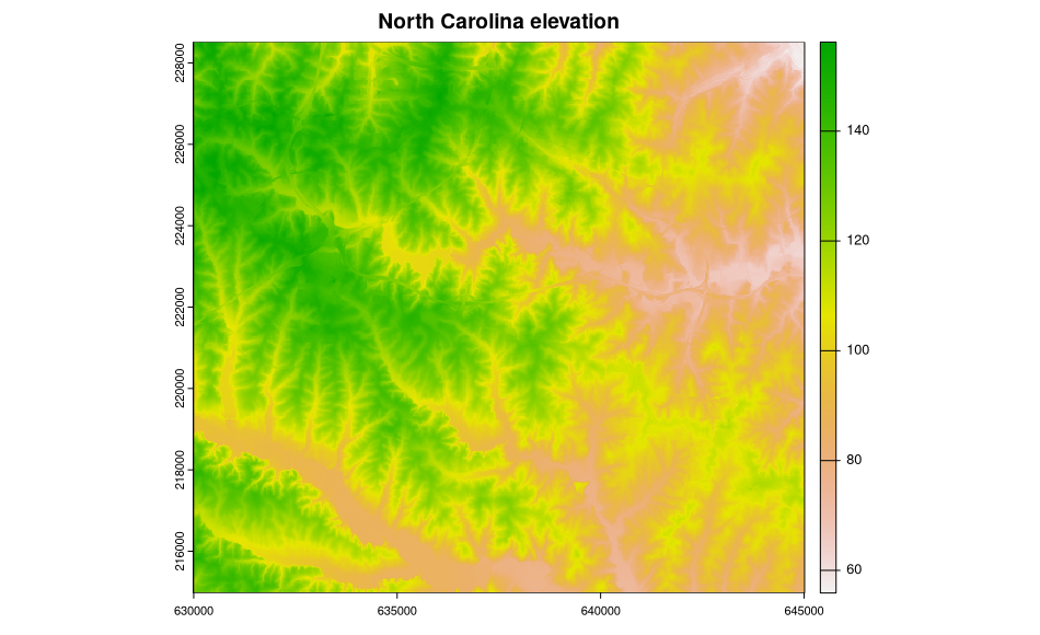
The metadata are accessed and available, but are not (yet) used to structure the sp class objects, in this case a SpatialGridDataFrame object filled with data from two North Carolina layers. Here is a plot of the elevation data:
> image(ncdata, attr = 2, col = terrain.colors(20))
Add a title to the plot:
> title("North Carolina elevation")

In addition, we can show what is going on inside the objects read into R:
> str(G)
List of 26
 $ DEBUG        : chr "0"
 $ LOCATION_NAME: chr "nc_spm_08_grass7"
 $ GISDBASE     : chr "/home/veroandreo/grassdata"
 $ MAPSET       : chr "PERMANENT"
 $ GUI          : chr "wxpython"
 $ projection   : chr "99"
 $ zone         : chr "0"
 $ n            : num 228500
 $ s            : num 215000
 $ w            : num 630000
 $ e            : num 645000
 $ t            : num 1
 $ b            : num 0
 $ nsres        : num 27.5
 $ nsres3       : num 10
 $ ewres        : num 37.5
 $ ewres3       : num 10
 $ tbres        : num 1
 $ rows         : int 491
 $ rows3        : int 1350
 $ cols         : int 400
 $ cols3        : int 1500
 $ depths       : int 1
 $ cells        : chr "196400"
 $ cells3       : chr "2025000"
 $ proj4        : chr "+proj=lcc +lat_1=36.16666666666666 +lat_2=34.33333333333334 +lat_0=33.75 +lon_0=-79 +x_0=609601.22 +y_0=0 +no_defs +a=6378137 +"| __truncated__
 - attr(*, "class")= chr "gmeta"
> summary(ncdata)
Object of class SpatialGridDataFrame
Coordinates:
        min    max
[1,] 630000 645000
[2,] 215000 228500
Is projected: TRUE
proj4string :
[+proj=lcc +lat_1=36.16666666666666 +lat_2=34.33333333333334
+lat_0=33.75 +lon_0=-79 +x_0=609601.22 +y_0=0 +no_defs +a=6378137
+rf=298.257222101 +towgs84=0.000,0.000,0.000 +to_meter=1]
Grid attributes:
  cellcentre.offset cellsize cells.dim
1          630018.8 37.50000       400
2          215013.7 27.49491       491
Data attributes:
   geology_30m      elevation
 CZfg_217:70381   Min.   : 55.92
 CZig_270:66861   1st Qu.: 94.78
 CZbg_405:24561   Median :108.88
 CZlg_262:19287   Mean   :110.38
 CZam_862: 6017   3rd Qu.:126.78
 CZbg_910: 4351   Max.   :156.25
 (Other) : 4942
Summarizing data
We can create a table of cell counts:
> table(ncdata$geology_30m)
| CZfg_217 | CZlg_262 | CZig_270 | CZbg_405 | CZve_583 | CZam_720 | CZg_766 | CZam_862 | CZbg_910 | Km_921 | CZbg_945 | CZam_946 | CZam_948 |
|---|---|---|---|---|---|---|---|---|---|---|---|---|
| 70381 | 19287 | 66861 | 24561 | 2089 | 467 | 691 | 6017 | 4351 | 1211 | 1 | 398 | 85 |
And compare with the equivalent GRASS module:
> execGRASS("r.stats", flags=c("c", "l"), parameters=list(input="geology_30m"), ignore.stderr=TRUE)
217 CZfg 70381
262 CZlg 19287
270 CZig 66861
405 CZbg 24561
583 CZve 2089
720 CZam 467
766 CZg 691
862 CZam 6017
910 CZbg 4351
921 Km 1211
945 CZbg 1
946 CZam 398
948 CZam 85
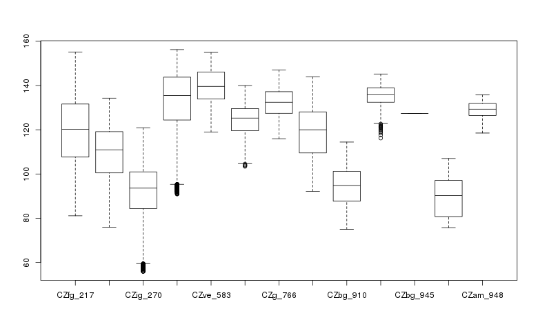
Create a box plot of geologic types at different elevations:
> boxplot(ncdata$elevation ~ ncdata$geology_30m, medlwd = 1)

Exporting data back to GRASS
Finally, a SpatialGridDataFrame object is written back to a GRASS raster map:
First prepare some data: (square root of elevation)
> ncdata$sqdem <- sqrt(ncdata$elevation)
Export data from R back into a GRASS raster map:
> writeRAST(ncdata, "sqdemNC", zcol="sqdem", ignore.stderr=TRUE)
Check that it imported into GRASS ok:
> execGRASS("r.info", parameters=list(map="sqdemNC"))
 +----------------------------------------------------------------------------+
 | Map:      sqdemNC                        Date: Sun Jul 19 13:06:34 2015    |
 | Mapset:   PERMANENT                      Login of Creator: veroandreo      |
 | Location: nc_spm_08_grass7                                                 |
 | DataBase: /home/veroandreo/grassdata                                       |
 | Title:     ( sqdemNC )                                                     |
 | Timestamp: none                                                            |
 |----------------------------------------------------------------------------|
 |                                                                            |
 |   Type of Map:  raster               Number of Categories: 0               |
 |   Data Type:    DCELL                                                      |
 |   Rows:         491                                                        |
 |   Columns:      400                                                        |
 |   Total Cells:  196400                                                     |
 |        Projection: Lambert Conformal Conic                                 |
 |            N:     228500    S: 215000.0002   Res: 27.49490794              |
 |            E:     645000    W:     630000   Res:  37.5                     |
 |   Range of data:    min = 7.47818253045085  max = 12.5000787351036         |
 |                                                                            |
 |   Data Description:                                                        |
 |    generated by r.in.bin                                                   |
 |                                                                            |
 |   Comments:                                                                |
 |                                                                            |
 +----------------------------------------------------------------------------+
Calling RStudio from a GRASS GIS session
If you are most used to run R through RStudio, but still want to have all GRASS data available for performing any analyses without loosing the possibility of still using GRASS command line, you can run:
GRASS> rstudio &
or, if you already are working on a certain RStudio project:
GRASS> rstudio /path/to/project/folder/ &
Then, you load rgrass7 library in your RStudio project
> library(rgrass7)
and you are ready to go.
GRASS within R
To call GRASS GIS 7 functionality from R, use the initGRASS() function to define the GRASS settings:
library(rgrass7)

# initialisation and the use of North Carolina sample dataset
initGRASS(gisBase = "/home/veroandreo/software/grass-7.0.svn", home = tempdir(),
          gisDbase = "/home/veroandreo/grassdata/",
          location = "nc_spm_08_grass7", mapset = "user1", SG="elevation",
          override = TRUE)

system("g.region -d")
# verify
gmeta()

ncdata <- readRAST(c("geology_30m", "elevation"), cat=c(TRUE, FALSE), ignore.stderr=TRUE, plugin=NULL)

summary(ncdata$geology_30m)
Run this script with
R CMD BATCH batch.R
This is not working at the moment
The result is (shorted here):
   cat batch.Rout

   R version 2.10.0 (2009-10-26)
   Copyright (C) 2009 The R Foundation for Statistical Computing
   ISBN 3-900051-07-0
   ...
   > library(rgrass7)
   Loading required package: sp
   Loading required package: rgdal
   Geospatial Data Abstraction Library extensions to R successfully loaded
   Loaded GDAL runtime: GDAL 1.7.2, released 2010/04/23
   Path to GDAL shared files: /usr/local/share/gdal
   Loaded PROJ.4 runtime: Rel. 4.7.1, 23 September 2009
   Path to PROJ.4 shared files: (autodetected)
   Loading required package: XML
   GRASS GIS interface loaded with GRASS version: (GRASS not running)
   >
   > # initialisation and the use of spearfish60 data
   > initGRASS(gisBase = "/usr/local/grass-6.4.1", home = tempdir(), gisDbase = "/home/neteler/grassdata/",
   +           location = "spearfish60", mapset = "user1", SG="elevation.dem", override = TRUE)
   gisdbase    /home/neteler/grassdata/
   location    spearfish60
   mapset      user1
   rows        477
   columns     634
   north       4928010
   south       4913700
   west        589980
   east        609000
   nsres       30
   ewres       30
   projection  +proj=utm +zone=13 +a=6378206.4 +rf=294.9786982 +no_defs
   +nadgrids=/usr/local/grass-6.4.1/etc/nad/conus +to_meter=1.0
   Warning messages:
   1: In dir.create(gisDbase) : '/home/neteler/grassdata' already exists
   2: In dir.create(loc_path) :
     '/home/neteler/grassdata//spearfish60' already exists
   >
   > system("g.region -d")
   > # verify
   > gmeta6()
   gisdbase    /home/neteler/grassdata/
   location    spearfish60
   mapset      user1
   rows        477
   columns     634
   north       4928010
   ...
   >
   > spear <- readRAST6(c("geology", "elevation.dem"),
   +           cat=c(TRUE, FALSE), ignore.stderr=TRUE,
   +           plugin=NULL)
   >
   > summary(spear$geology)
   metamorphic  transition     igneous   sandstone   limestone       shale
         11693         142       36534       74959       61355       46423
   sandy shale    claysand        sand        NA's
         11266       14535       36561        8950
   >
   >
   > proc.time()
      user  system elapsed
     2.891   0.492   3.412