R statistics/spgrass6: Difference between revisions
Veroandreo (talk | contribs) (→R within GRASS: more formatting) |
Veroandreo (talk | contribs) (→GRASS within R: more formatting) |
||
| Line 249: | Line 249: | ||
To call GRASS GIS 6 functionality from R, use the initGRASS() function to define the GRASS settings: | To call GRASS GIS 6 functionality from R, use the initGRASS() function to define the GRASS settings: | ||
<source lang="rsplus"> | |||
library(spgrass6) | |||
# initialisation and the use of spearfish60 data | # initialisation and the use of spearfish60 data | ||
initGRASS(gisBase = "/usr/local/grass-6.4.1", home = tempdir(), | |||
gisDbase = "/home/neteler/grassdata/", | gisDbase = "/home/neteler/grassdata/", | ||
location = "spearfish60", mapset = "user1", SG="elevation.dem", | location = "spearfish60", mapset = "user1", SG="elevation.dem", | ||
| Line 266: | Line 267: | ||
summary(spear$geology) | summary(spear$geology) | ||
</source> | |||
Run this script with | Run this script with | ||
<source lang="bash"> | |||
R CMD BATCH batch.R | |||
</source> | |||
The result is (shorted here): | The result is (shorted here): | ||
<source lang="bash"> | |||
cat batch.Rout | |||
</source> | |||
<source lang="rsplus"> | |||
R version 2.10.0 (2009-10-26) | R version 2.10.0 (2009-10-26) | ||
Copyright (C) 2009 The R Foundation for Statistical Computing | Copyright (C) 2009 The R Foundation for Statistical Computing | ||
| Line 336: | Line 343: | ||
user system elapsed | user system elapsed | ||
2.891 0.492 3.412 | 2.891 0.492 3.412 | ||
</source> | |||
[[Category:FAQ]] | [[Category:FAQ]] | ||
Latest revision as of 18:02, 15 September 2016
This page refers to the usage of R within a GRASS GIS 6 session and the use of GRASS GIS 6 within an R session. (see also R_statistics/rgrass7)
R within GRASS
Startup
- First start a GRASS session. Then, at the GRASS command line start R.
- In this example we will use the sample Spearfish dataset.
Reset the region settings to the defaults
GRASS> g.region -d
Launch R from the GRASS prompt
GRASS> R
Load the spgrass6 library:
library(spgrass6)Get the GRASS environment (mapset, region, map projection, etc.); you can display the metadata for your location by printing G:
G <- gmeta6()Listing of existing maps
List available vector maps:
execGRASS("g.list", parameters = list(type = "vect"))List selected vector maps (wildcard):
execGRASS("g.list", parameters = list(type = "vect", pattern = "precip*"))Save selected vector maps into R vector:
my_vmaps <- execGRASS("g.list", parameters = list(type = "vect", pattern = "precip*"))
attributes(my_vmaps)
attributes(my_vmaps)$resOut
List available raster maps:
execGRASS("g.list", parameters = list(type = "rast"))List selected raster maps (wildcard):
execGRASS("g.list", parameters = list(type = "rast", pattern = "lsat7_2000*"))Reading in data
Read in two raster maps (Spearfish sample dataset):
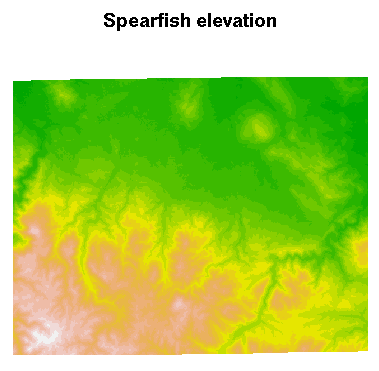
spear <- readRAST6(c("geology", "elevation.dem"), cat=c(TRUE, FALSE), ignore.stderr=TRUE, plugin=NULL)The metadata are accessed and available, but are not (yet) used to structure the sp class objects, here a SpatialGridDataFrame object filled with data from two Spearfish layers. Here is a plot of the elevation data:
image(spear, attr = 2, col = terrain.colors(20))Add a title to the plot:
title("Spearfish elevation")
In addition, we can show what is going on inside the objects read into R:
str(G)
List of 26
 $ GISDBASE     : chr "/home/rsb/topics/grassdata"
 $ LOCATION_NAME: chr "spearfish57"
 $ MAPSET       : chr "rsb"
 $ DEBUG        : chr "0"
 $ GRASS_GUI    : chr "text"
 $ projection   : chr "1 (UTM)"
 $ zone         : chr "13"
 $ datum        : chr "nad27"
 $ ellipsoid    : chr "clark66"
 $ north        : num 4928010
 $ south        : num 4913700
 $ west         : num 589980
 $ east         : num 609000
 $ top          : num 1
 $ bottom       : num 0
 $ nsres        : num 30
 $ nsres3       : num 30
 $ ewres        : num 30
 $ ewres3       : num 30
 $ tbres        : num 1
 $ rows         : int 477
 $ rows3        : int 477
 $ cols         : int 634
 $ cols3        : int 634
 $ depths       : int 1
 $ proj4        : chr "+proj=utm +zone=13 +a=6378206.4 +rf=294.9786982 +no_defs +nadgrids=/home/rsb/topics/grass61/grass-6.1.cvs/etc/nad/conus"

summary(spear)
Object of class SpatialGridDataFrame
Coordinates:
              min     max
coords.x1  589980  609000
coords.x2 4913700 4928010
Is projected: TRUE
proj4string : [+proj=utm +zone=13 +a=6378206.4 +rf=294.9786982 +no_defs +nadgrids=/home/rsb/topics/grass61/grass-6.1.cvs/etc/nad/conus]
Number of points: 2
Grid attributes:
  cellcentre.offset cellsize cells.dim
1            589995       30       634
2           4913715       30       477
Data attributes:
      geology      elevation.dem
 sandstone:74959   Min.   : 1066
 limestone:61355   1st Qu.: 1200
 shale    :46423   Median : 1316
 sand     :36561   Mean   : 1354
 igneous  :36534   3rd Qu.: 1488
 (Other)  :37636   Max.   : 1840
 NA's     : 8950   NA's   :10101
Summarizing data
We can create a table of cell counts:
table(spear$geology)| metamorphic | transition | igneous | sandstone | limestone | shale | sandy shale | claysand | sand |
|---|---|---|---|---|---|---|---|---|
| 11693 | 142 | 36534 | 74959 | 61355 | 46423 | 11266 | 14535 | 36561 |
And compare with the equivalent GRASS module:
execGRASS("r.stats", flags=c("c", "l"), parameters=list(input="geology"), ignore.stderr=TRUE)1 metamorphic 11693 2 transition 142 3 igneous 36534 4 sandstone 74959 5 limestone 61355 6 shale 46423 7 sandy shale 11266 8 claysand 14535 9 sand 36561 * no data 8950
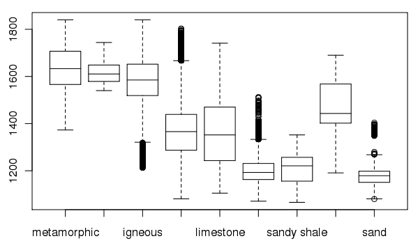
Create a box plot of geologic types at different elevations:
boxplot(spear$elevation.dem ~ spear$geology, medlwd = 1)
Exporting data back to GRASS
Finally, a SpatialGridDataFrame object is written back to a GRASS raster map:
First prepare some data: (square root of elevation)
spear$sqdem <- sqrt(spear$elevation.dem)Export data from R back into a GRASS raster map:
writeRAST6(spear, "sqdemSP", zcol="sqdem", ignore.stderr=TRUE)Check that it imported into GRASS ok:
execGRASS("r.info", parameters=list(map="sqdemSP"))+----------------------------------------------------------------------------+ | Layer: sqdemSP Date: Sun May 14 21:59:26 2006 | | Mapset: rsb Login of Creator: rsb | | Location: spearfish57 | | DataBase: /home/rsb/topics/grassdata | | Title: ( sqdemSP ) | |----------------------------------------------------------------------------| | | | Type of Map: raster Number of Categories: 255 | | Data Type: FCELL | | Rows: 477 | | Columns: 634 | | Total Cells: 302418 | | Projection: UTM (zone 13) | | N: 4928010 S: 4913700 Res: 30 | | E: 609000 W: 589980 Res: 30 | | Range of data: min = 32.649654 max = 42.895222 | | | | Data Source: | | | | | | | | Data Description: | | generated by r.in.gdal | | | | | +----------------------------------------------------------------------------+
v.krige usage example
v.krige is a GRASS python script (Addon) which performs kriging operations in the GRASS environment, using R functions for the back-end interpolation. It is present in GRASS 6.5svn, and further developed in GRASS 7svn. It requires a number of dependencies: python-rpy2 (needs to be "Rpy2", "Rpy" will not do unless it is rpy 2.x), then the following R-CRAN packages:
* gstat, spgrass6 (as above)
 install.packages(c("gstat","spgrass6"))
* maptools
 install.packages("maptools")
* automap (optional), with gpclib (or rgeos)
 install.packages("automap")
 install.packages("rgeos")
GRASS within R
To call GRASS GIS 6 functionality from R, use the initGRASS() function to define the GRASS settings:
    library(spgrass6)

    # initialisation and the use of spearfish60 data
    initGRASS(gisBase = "/usr/local/grass-6.4.1", home = tempdir(),
              gisDbase = "/home/neteler/grassdata/",
              location = "spearfish60", mapset = "user1", SG="elevation.dem",
              override = TRUE)

    system("g.region -d")
    # verify
    gmeta6()

    spear <- readRAST6(c("geology", "elevation.dem"),
              cat=c(TRUE, FALSE), ignore.stderr=TRUE,
              plugin=NULL)

    summary(spear$geology)
Run this script with
R CMD BATCH batch.R
The result is (shorted here):
cat batch.Rout
    R version 2.10.0 (2009-10-26)
    Copyright (C) 2009 The R Foundation for Statistical Computing
    ISBN 3-900051-07-0
    ...
    > library(spgrass6)
    Loading required package: sp
    Loading required package: rgdal
    Geospatial Data Abstraction Library extensions to R successfully loaded
    Loaded GDAL runtime: GDAL 1.7.2, released 2010/04/23
    Path to GDAL shared files: /usr/local/share/gdal
    Loaded PROJ.4 runtime: Rel. 4.7.1, 23 September 2009
    Path to PROJ.4 shared files: (autodetected)
    Loading required package: XML
    GRASS GIS interface loaded with GRASS version: (GRASS not running)
    >
    > # initialisation and the use of spearfish60 data
    > initGRASS(gisBase = "/usr/local/grass-6.4.1", home = tempdir(), gisDbase = "/home/neteler/grassdata/",
    +           location = "spearfish60", mapset = "user1", SG="elevation.dem", override = TRUE)
    gisdbase    /home/neteler/grassdata/
    location    spearfish60
    mapset      user1
    rows        477
    columns     634
    north       4928010
    south       4913700
    west        589980
    east        609000
    nsres       30
    ewres       30
    projection  +proj=utm +zone=13 +a=6378206.4 +rf=294.9786982 +no_defs
    +nadgrids=/usr/local/grass-6.4.1/etc/nad/conus +to_meter=1.0
    Warning messages:
    1: In dir.create(gisDbase) : '/home/neteler/grassdata' already exists
    2: In dir.create(loc_path) :
      '/home/neteler/grassdata//spearfish60' already exists
    >
    > system("g.region -d")
    > # verify
    > gmeta6()
    gisdbase    /home/neteler/grassdata/
    location    spearfish60
    mapset      user1
    rows        477
    columns     634
    north       4928010
    ...
    >
    > spear <- readRAST6(c("geology", "elevation.dem"),
    +           cat=c(TRUE, FALSE), ignore.stderr=TRUE,
    +           plugin=NULL)
    >
    > summary(spear$geology)
    metamorphic  transition     igneous   sandstone   limestone       shale
          11693         142       36534       74959       61355       46423
    sandy shale    claysand        sand        NA's
          11266       14535       36561        8950
    >
    >
    > proc.time()
       user  system elapsed
      2.891   0.492   3.412