Help with 3D
Raster 2.5D Surface
This is the "typical" case, and most GRASS r.* modules work in this mode. The GIS layer is defined by north,south,east,west and the raster map's cell values represent the elevation.
Snippet from the Wikipedia definition: "The idea is that the program's canvas represents a normal 2D painting surface, but that the data structure that holds the pixel information is also able to store information regarding z-index (depth) as well as other information such as material settings, specularity, etc. With this data it is thus possible to simulate lighting, shadows, and so on."
Horizontal (2D) region settings are handled by the g.region module. The third dimension is unbound.
It is possible to make a 4D (change with time) visualization using the NVIZ software's animation panels and movie making facility.
2.5D rasters may be visualized in 3D with GRASS's NVIZ program, or as a shaded relief in 2D space with the r.shaded.relief module.
Screenshots
Example
(spearfish dataset)
g.region rast=elevation.10m
nviz elev=elevation.10m
Raster 3D Volumes (voxels)
Support for 3D rasters (voxels) is relatively new in GRASS and is primarily handled by the r3.* modules. A 3D raster can be thought of as a stack of 2D raster maps forming a 3D cube of data cells.
Screenshots
- Chesapeake Bay Nitrogen (4D) from NCSU GMS Lab (Mitasova et al.)
Region settings
Region settings are handled by the g.region module. Special 3D raster controls for g.region include:
-3 flag:  Prints 3D settings
      t   Value for the top edge
      b   Value for the bottom edge
   res3   3D grid resolution (north-south, east-west and top-bottom)
  tbres   Top-bottom grid resolution 3D
and
rast3d Set region to match this 3D raster map (both 2D and 3D values)
Examples
- Custom volume creation. Here is a small Octave (Matlab) script to create a text file suitable for loading as a 3D raster with r3.in.ascii.
- Here is the file that this script creates:
x= y= z= 50;

cd ~/grass/
fp = fopen('vox_data50.txt', 'wt')

fprintf(fp, 'north: %d\n', y);
fprintf(fp, 'south: 0\n');
fprintf(fp, 'east: %d\n', x);
fprintf(fp, 'west: 0\n');
fprintf(fp, 'top: %d\n', z);
fprintf(fp, 'bottom: 0\n');
fprintf(fp, 'rows: %d\n', y);
fprintf(fp, 'cols: %d\n', x);
fprintf(fp, 'levels: %d\n', z);

for dep = 1:z
  for row = 1:y
    for col = 1:x
       fprintf(fp, '%.4f', col + (row^2 /2) + dep^2 );
       if(col < 50)
          fprintf(fp, ' ');
       end
    end
    fprintf(fp, '\n');
  end
  disp(['dep ' num2str(dep)])
  fflush(stdout);
end
fclose(fp)
Load the data with:
r3.in.ascii in=vox_data50.txt out=vox50
display isosurfaces with:
g.region rast3d=vox50
nviz -q
Panel->Raster volumes
[New] vox50
Isosurface [Add] [New Constant] 500 [Accept]
 (repeat for 1000,2000,3000)
Change main view height to 125.00 (manual entry)
extract a slice to a 2D raster map with:
g.region t=26.0 b=25.0
r3.to.rast in=vox50 out=vox50x
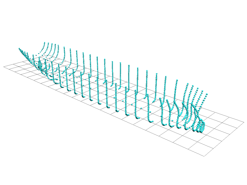
Vector 3D point data
- v.in.ascii -z format=point
- r.in.xyz
Screenshot
3D points defining the hull of a ship, visualized using NVIZ

Example
TODO: import star guide and display using NVIZ
Vector 3D polygons
intro
- faces
- kernel
- GRASS ascii format definition
- "v.in.ascii -z"
- Visualization with NVIZ: must be placed on a raster surface or constant surface. It may be useful to set the transparency attribute of the raster surface to something unobtrusive.
Screenshots
Example
pyramid: the following is an example of 3D vector surfaces in GRASS standard ascii format. load with v.in.ascii.
# 3D Pyramid in GRASS:  (kernel currently unused?)
#  v.in.ascii in=pyramid.vasc out=pyramid_3d format=standard -nz
#  g.region n=150 s=-50 w=-50 e=150 res=10
#  r.mapcalc one=1
#  nviz elev=one vect=pyramid_3d
#
#  tip: in nviz try setting the raster surface transparency to 50%
#
F 5
 0 0 10
 0 100 10
 100 100 10
 100 0 10
 0 0 10
F 4
 0 0 10
 50 50 80
 100 0 10
 0 0 10
F 4
 0 100 10
 50 50 80
 0 0 10
 0 100 10
F 4
 100 100 10
 50 50 80
 0 100 10
 100 100 10
F 4
 100 0 10
 50 50 80
 100 100 10
 100 0 10
K 1 1
 40 50 40
 1 1
Visualization Tools
- NVIZ: GRASS's own visualization suite
- output to VTK
- output to POVray
- output to V5D