Population Genetics and GIS
Applying Population Genetics, Habitat Suitability Modeling and GIS to create predicted migration corridors for New World Screw-worm
Background
New world Screw-worm Cochliomyia hominivorax (NWS) is a well known insect pest in South and North America, causing extensive damage to livestock. The females lay eggs into small wounds in warm-blooded vertebrate and the larvae then burrow into the tissue. This injury, known as myasis, weakens the animal, lowers production, and sometimes is severe enough to lead to death of the animal. The "cousin" of NWS, the Old World Screw-worm Chrysomya bezziana (OWS) causes similar effects throughout the Middle East and South East Asia.
Typically these insect pests are treated by spraying the livestock directly with pesticides. However they are an ideal candidate for treatment by Sterile Insect Technique (SIT) in the context of an Area-Wide pest management program. See the Joint FAO/IAEA program. An SIT based program requires releasing huge numbers of sterilized male flies throughout the grazing lands, so that the female flies do not encounter a wild male, thus leading to a substantial reduction in the population within a few generations. The method is cost effective when the treated area actually is infested or potentially can be infested with screw-worm. So a successful SIT treatment plan depends on a good understanding of the distribution and possible migration of the pest. This research attempts to address that very question. By merging population genetics and a species habitat model through the use of GIS tools, a procedure is suggested which leads to a geographic data layer representing possible migration corridors of the insect. These corridors are created by combining genetic distance data with environmental data using GRASS GIS.
Genetics
In this research, we used the pairwise Fst matrix estimated in Fresia et al. 2011. (full text availble on request) as the genetic distance between samples from all pairs of locations. A total of 227 mitochondrial haplotypes were identified in 282 individuals collected from 29 locations throughout S. America and grouped into two "geographic groups". From the matrix, those pairs with Fst=0 (genetically identical samples) were retained for further work. This Fst=0 value was chosen based on the dispersal capability of the NWS and can be adjusted in any particular case.
Habitat Suitability Model
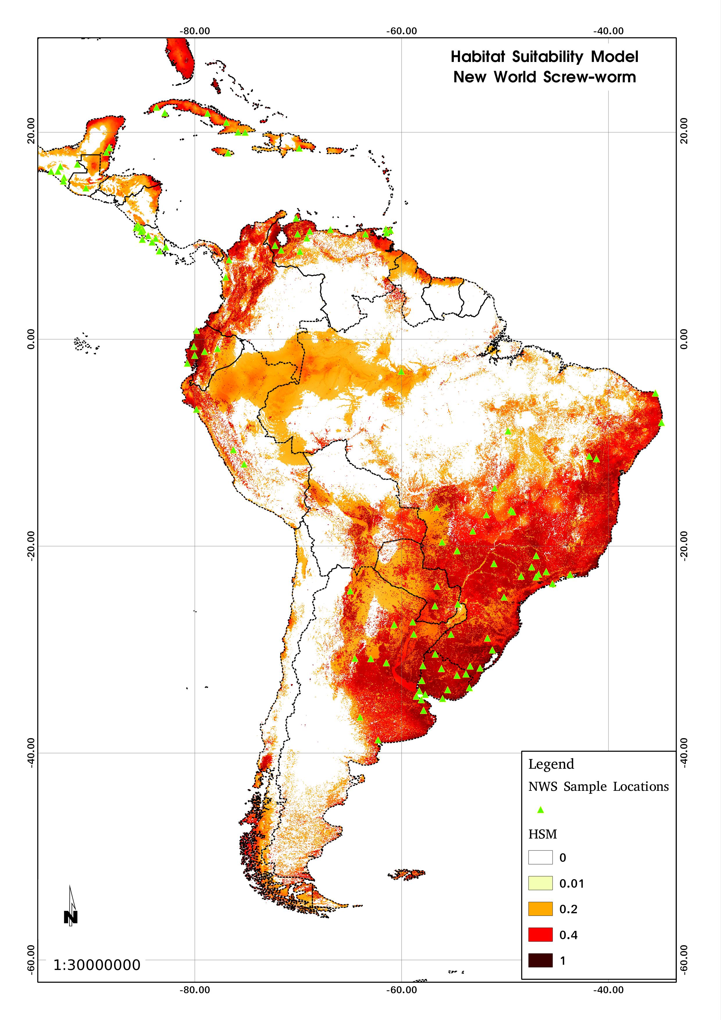
The presence only algorithm employed by MaxEnt ( software for species habitat modeling ) was used to create a Habitat Suitability Model (HSM). Environmental predictors were chosen from the BioCLIM data, as well as elevation, landcover (the glc2000 dataset ) and livestock density from the FAO Gridded Livestock of the World data layer. The resulting raster showed the habitat suitability of the NWS based on environmental conditions.
GIS
GRASS-GIS was chosen to perform the spatial analyses due to the variety of available modules, and ease of scripting the procedures. The steps to merge the genetic distance data with the HSM are itemized below. The script used is available online here.
Two text files in CSV format were prepared in advance, to be read by the GRASS script:
- A list of the locations, with location code and Lon/Lat coordinates for each location, as "localities.csv"
- A list of the pairs of location codes for which the Fst value was zero, as "Fst_zero.csv"
The procedure is broken into four steps:
Read in the HSM raster
The HSM raster is inverted to create a friction raster. This is done simply with r.in.gdal, and an r.mapcalc expression:
r.in.gdal in=hsm.tiff out=hsm
g.region -p rast=hsm
r.mapcalc friction="1.0-hsm"
Create cost maps for each of the locations based on the friction raster
The GRASS module r.cost was run in a loop, reading each location code, and its coordinates from the localities.csv ASCII text file. The code run in each cycle of the loop consisted of:
r.cost --verbose --overwrite input=friction out=cost_"$code" coord="$lon,$lat";
By looping through all the locations, cost rasters were created which represent the difficulty, or cost (from the friction map) to reach each of the locations from any other pixel in the region. This "difficulty" is drawn from the original environmental layers as represented in the habitiat suitability model. In the resulting cost raster, pixels with a low value are those where is would be "easy" for an insect to migrate to, from the given location. Pixels with a high value represent locations to which it's unlikely that an insect would migrate.
Combine the cost rasters
Use matrix addition to combine two cost rasters, considering only those pairs of locations for which the genetic distance was close (Fst = 0). The script loops through pairs of locations read from the Fst_zero.csv ASCII text file. In addition to adding the rasters, the result is used to create a reclassed raster as follows:
- The minimum value from the combined raster is given value 3.
- Values up to 2% higher than the minimum are given value 2
- Values from 2% to 5% higher than the minimum are given value 1
- all other values are set to null
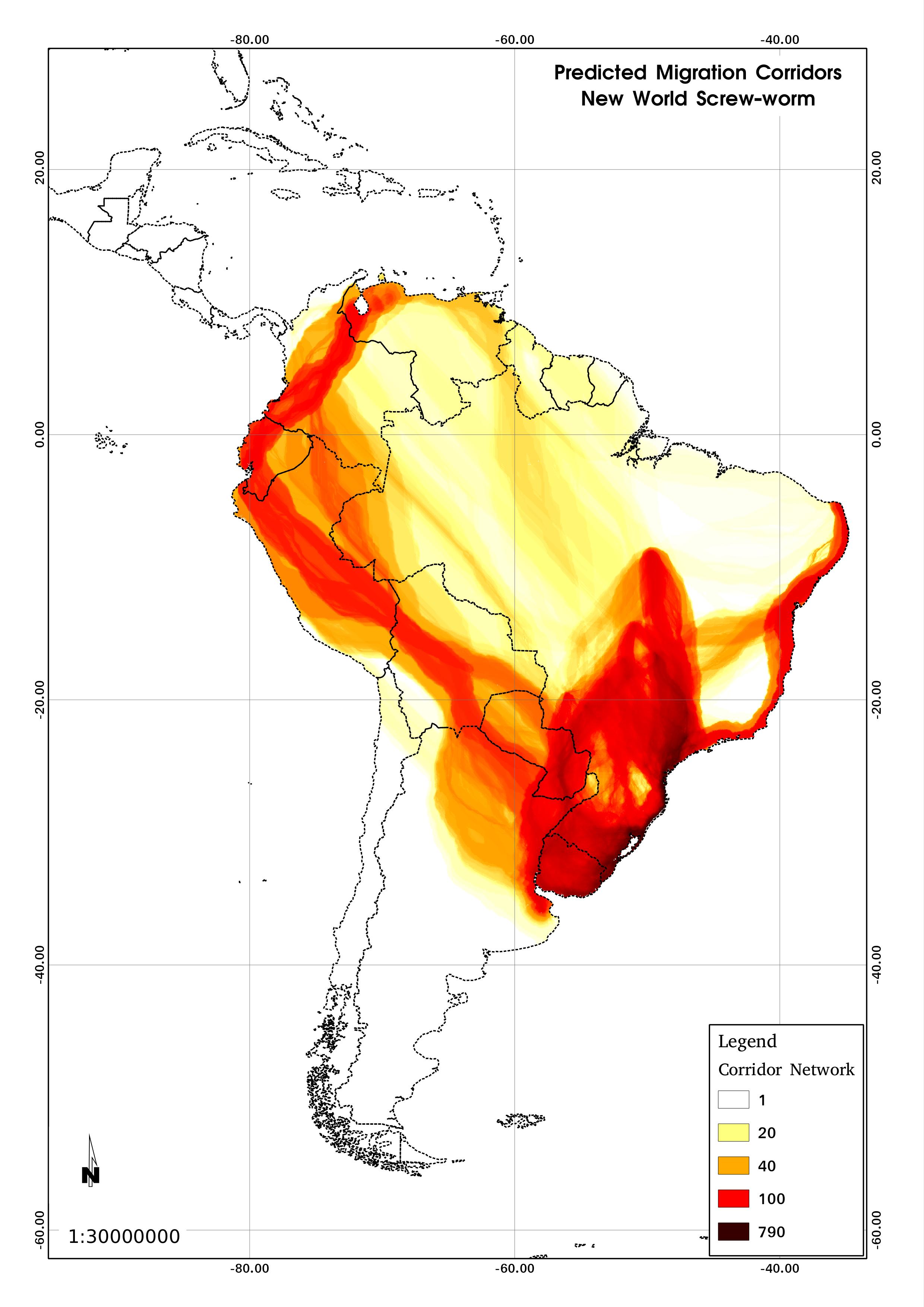
This new reclass raster essentially creates a least cost path (LCP), or corridor between pairs of locations. This LCP corridor merges the environmental connectivity, and the genetic distance between locations. A LCP raster is created for each pair of points with the following code:
r.mapcalc corridor_"$loc1"_"$loc2"="round(cost_"$loc1" + cost_"$loc2")"
# Save variables for reclass from r.univar
min=`r.univar -g corridor_"$loc1"_"$loc2" | grep min | cut -d= -f2`
two_percent=`echo $min*1.02/1 | bc`
five_percent=`echo $min*1.05/1 | bc`
 # Create the reclass rules file for a specific pair of locations
cat << EOF > "$loc1"_"$loc2"_rules.txt
$min                    = 3             Minimum
$min thru $two_percent  = 2             Two percent
$two_percent thru $five_percent = 1     Five percent
*                       = NULL          NULL
end
EOF
# Create the reclass raster for a specific pair using the new reclass rules file
r.reclass --overwrite input=corridor_"$loc1"_"$loc2" output=lcp_"$loc1"_"$loc2" rule="$loc1"_"$loc2"_rules.txt title="$loc1 - $loc2   Least Cost Path"
Finally merge all reclass rasters
Create an overall LCP raster for the whole region by summing all the reclass maps, showing possible migration corridors.
lcp_maps=`g.mlist type=rast pattern="lcp*" separator=,`
r.series --overwrite input=$lcp_maps output=lcp_merged method=sum
Samples
Here are two sample maps of HSM and LCP corridors.resulting predicted migration corridors.


Map 1: the HSM for New World Screw-worm in S. America
Map 2: the resulting predicted migration corridors
Discussion
The corridor map above, and similar results, show good correlation with the accepted understanding of NSW migration in South America. This match between assumed movement of the insect, and the resulting corridor map increases our confidence in the validity of the procedure. Furthermore, each of the three components of the method outlined above - genetic differentiation, habitat suitability, and least cost path analysis - is flexible. Many adjustments can be applied to adapt the procedure to differing circumstances and other species. We hope therefore that other researchers will adopt the method, and report similar encouraging results.
Regarding NWS and OWS, we believe that this technique could become an integral part of any Area-Wide treatment program, employing SIT to reduce the insect population while avoiding repeated pesticide applications. Infestation can be reduced dramatically, improving livestock production, and allowing expansion of herds into new grazing areas without concern for renewed screw-worm attacks. An analysis of migration corridors will ensure efficient and effective use of SIT, making it a viable as well as safe tool for fighting myasis.
Authors
- Pablo Fresia, pfresia at gmail com
- Micha Silver, micha at arava co il