Temporal data processing/GRASS R raster time series processing
GRASS-R / R-GRASS for raster time series processing
This little example will guide you through the steps to export a Spatio-Temporal Raster Dataset (strds) stored in GRASS, import it into R, prepare the data properly to use the Data INterpolation Empirical Orthogonal Functions algorithm (DINEOF) and, after running it, rebuild your raster time series, export it and import the new strds into GRASS.
We will use North Carolina climatic data already available as a GRASS location. You can get it here. If not done yet, you need to unzip the file and paste into your GRASS database folder (usually named grassdata).
Shall we start?
1. In GRASS GIS
- Open GRASS in the location/mapset of interest
grass70 $HOME/grassdata/nc_climate_spm_2000_2012/climate_1970_2012/
- List raster maps with pattern=*tempmean
g.list type=raster pattern=*tempmean
- Create a strds with mean temperature maps: t.create
t.create output=tempmean type=strds temporaltype=absolute \
    title="Average temperature" description="Monthly temperature average in NC [deg C]"
- Register maps in the strds (t.register), list the strds (t.list) and obtain general information for a particular space-time dataset (t.info). More details about different options to register maps in strds can be found in the dedicated map registration wiki.
t.register -i input=tempmean type=raster start=2000-01-01 increment="1 months" \
    maps=`g.list type=raster pattern=*tempmean separator=comma`

t.list type=strds

t.info input=tempmean
- List maps and check basic statistics of the strds: t.rast.list and t.rast.univar
t.rast.list input=tempmean

t.rast.univar input=tempmean
- Export out of GRASS: t.rast.export
As said before, we will use DINEOF as gap-filling technique. This method is not (yet) available in GRASS GIS, so we need to export the raster time series. To export only a spatial subset of the raster maps, we set region to the default North Carolina computational region and then we use t.rast.export to export our strds.
# set default region
g.region -d

t.rast.export input=tempmean output=tempmean4R.tar.gzip compression=gzip
2. Moving to R
- From the GRASS console, open R (or rstudio)
Note that you can directly open a project in which you were already working (as in the example above) or just type R or rstudio followed by & so you do not loose the command prompt in GRASS console. More details and examples of how to use R or rstudio within a GRASS session can be found in the dedicated wiki. Look for R within GRASS and Rstudio within GRASS sections.
rstudio $HOME/Documents/foss4g_bonn/ts_grass_r &
Once in R, we first load the rgrass7 package. This library provides the interface with GRASS GIS 7. We will also check some basic information about the session.
# Load rgrass7 package
library(rgrass7)

# Check GRASS environment
genv <- gmeta()
genv
gisdbase    /home/veroandreo/grassdata
location    nc_climate_spm_2000_2012
mapset      climate_1970_2012
rows        104
columns     139
north       260500
south       208500
west        624500
east        694000
nsres       500
ewres       500
projection  +proj=lcc +lat_1=36.16666666666666 +lat_2=34.33333333333334 +lat_0=33.75
+lon_0=-79 +x_0=609601.22 +y_0=0 +no_defs +a=6378137 +rf=298.257222101
+towgs84=0.000,0.000,0.000 +to_meter=1
This gives us information about projection and region settings, among other things, that we will need afterwards (see below).
Given that neither GRASS temporal modules nor GRASS space time data sets are (yet) enabled/implemented in R, when you need to process a time series that you have in GRASS DB you need to export all maps and then read them into R. Therefore, we need to load the following packages, too:
# Load other required packages
library(spacetime)
library(raster)
library(rgdal)
Now, we read the strds exported from GRASS into R with the function read.tgrass from spacetime package.
# Import strds into R
tempmean_in_R <- read.tgrass("tempmean4R.tar.gzip", localName = FALSE, useTempDir = FALSE)
Note that R imports our exported strds as a RasterStack. Let us see if all is there:
# Get information about the RasterStack
class(tempmean_in_R)
[1] "RasterStack"
attr(,"package")
[1] "raster"
# Dimensions
> dim(tempmean_in_R)
[1] 104 139 156
We can also ask summaries of particular layers in the stack or of the whole RasterStack.
# Summary of the first layer
summary(tempmean_in_R[[1]])
        X2000_01_tempmean
Min.             2.833784
1st Qu.          3.667942
Median           3.936594
3rd Qu.          4.132093
Max.             4.496206
NA's             0.000000

# Summary of the RasterStack
summary(tempmean_in_R)
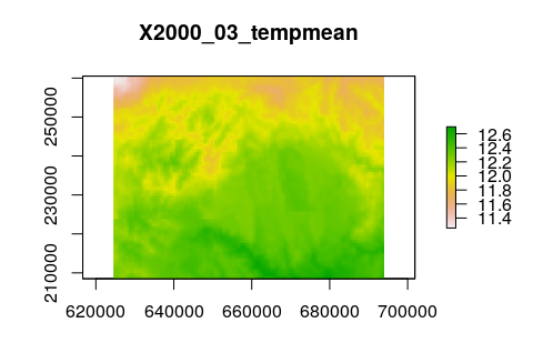
And, of course, we may also plot a certain layer.
# Plot 3rd layer in the stack
plot(tempmean_in_R,3)
For most methods in R (For example: Theil-Sen slope, fft, dineof), we will need to transform our RasterStack into a matrix or data.frame. In the particular case of this example, we need to transform our RasterStack into a matrix mxt, with m = maps and t = time, i.e.: in this matrix we have our maps as rows and time in columns. Therefore, in each column we have the time series for a given pixel. Let us start, then.
# RasterStack to matrix (this gives us maps as columns and time in rows)
txm_tempmean <- as.matrix(tempmean_in_R)
dim(txm_tempmean)
[1] 14456   156

# Transpose matrix (we need time in columns and maps unfolded in rows)
mxt_tempmean <- t(txm_tempmean)
dim(mxt_tempmean)
[1]   156 14456
All the point of DINEOF is gap-filling. However, as our sample dataset comes from interpolations of weather stations, we do not have such gaps...
# Check for gaps in data
sum(is.na(mxt_tempmean))
[1] 0
So, for the purpose of this example, we will create them.
# Create some holes.
# Total pixel counts: 14456*156=2255136
# NULL values must appear as NaN
set.seed(46)
n = 400000
mxt_tempmean[mysamples <- sample(length(mxt_tempmean), n)] <- NaN
sum(is.na(mxt_tempmean))
[1] 400000
Now we are ready to use DINEOF to fill our gappy data. You can find more info about DINEOF in the official site. However, the R package providing DINEOF is called sinkr and can be installed from here.
# Load library containing dineof function and other required libraries
library(sinkr)
library(irlba)
library(Matrix)
# or, download the dineof function from the repository and source it:
# source('dineof.r')

# Run the algorithm - default settings
result_tempmean <- dineof(mxt_tempmean)
The result_tempmean object is a list with all results from dineof. You may investigate yourself, try with other settings and compare results.
# Explore what's inside
names(result_tempmean)
[1] "Xa"    "n.eof" "RMS"   "NEOF"
For the purpose of this example, we will only extract the reconstructed spatio-temporal matrix and display it:
# Extract gap-filled matrix
tempmean_new <- result_tempmean$Xa

# Set color palette
library(RColorBrewer)
pal <- colorRampPalette(c("blue", "cyan", "yellow", "red"))

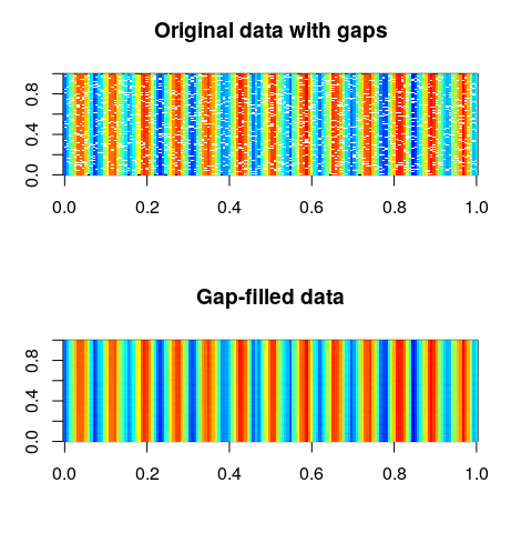
# Display the gappy and gap-filled spatio-temporal matrices
par(mfrow = c(2,1))
image(mxt_tempmean, col = pal(100), main = "Original data with gaps")
image(tempmean_new, col = pal(100), main = "Gap-filled data")

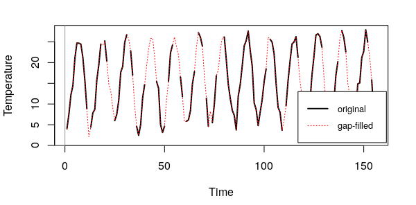
And we want to see how the time series of a particular pixel is reconstructed. Therefore, we just need to plot all the rows in a certain column. Do you remember how our matrix was formed?
# Plot the time series of a single pixel from both matrices
pixel <- 10000
ylim <- range(c(mxt_tempmean[,pixel], tempmean_new[,pixel]), na.rm = TRUE)
plot(mxt_tempmean[,pixel], t = "l", ylim = ylim, lwd = 2, ylab = "Temperature", xlab = "Time")
lines(tempmean_new[,pixel], col = 2, lty = 3)
legend(123, 13, c("original","gap-filled"), lty = c(1,3), lwd = c(2,1), col = c(1,2), cex = 0.8)
abline(h = 0, v = 0, col = "gray60")

Let us assume that we are happy with the result, we need now to go back to a strds format. We need to rebuild the raster time series starting from a matrix mxt. For that, we first create empty rasters of the same dimensions of our original raster maps and then, we fill them with each row of the gap-filled matrix. What we obtain then is a list of rasters. Let's see:
# Create raster objects to fill with data from tempmean_new
tempmean_2_grass <- raster(nrows = 104, ncols = 139,
           xmn = 624500, xmx = 694000,
           ymn = 208500, ymx = 260500,
           crs = tempmean_in_R)
dim(tempmean_2_grass)
[1] 104 139   1

# Extract data from each row of ''tempmean_new'' and build up a raster layer
# Output: list of rasters
tempmean_new_rl <- lapply(1:nrow(tempmean_new), function(i) {
  setValues(tempmean_2_grass, tempmean_new[i,])
  } )
length(tempmean_new_rl)
[1] 156
dim(tempmean_new_rl[[3]])
[1] 104 139   1

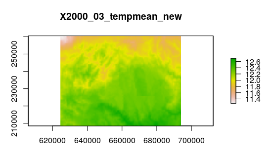
# Plot a raster layer in the list
plot(tempmean_new_rl[[3]], main="X2000_03_tempmean_new")

You can compare with layer 3 in the original data.
plot(tempmean_in_R,3)Well, so far we have a list of rasters. But to export them and import them back into GRASS, we need again a RasterStack.
# rebuild RasterStack
tempmean_new_rs <- stack(tempmean_new_rl)
Not only a RasterStack, but we need to specify the temporal dimension, i.e.: we need to add time to the RasterStack.
time_4_new_rs <- seq(as.Date("2001-01-01"), as.Date("2012-12-01"))
tempmean_new_rs_and_time <- setZ(tempmean_new_rs, time_4_new_rs, name="time")
Finally, we export the RasterStack to GRASS with the write.tgrass function from spacetime package.
write.tgrass(tempmean_new_rs_and_time, "tempmean_new_from_R.tar.gzip")3. Back to GRASS
Now, switch back to GRASS console and import the strds with t.rast.import. This command will create a strds and register all maps in it.
t.rast.import input=tempmean_new_from_R.tar.gz output=tempmean_dineof base=tempmean_dineof extrdir=/tmp
Enjoy!