LIDAR

LIDAR and Multi-beam Swath bathymetry data

Modules

Import

• r.in.xyz - Create a raster map from an assemblage of many coordinates using univariate statistics.
  (example)

• v.in.ascii - Import data from an ASCII file to GRASS vector format.
  Limited to a few million data points unless topology and database creation is skipped with the -bt flags

Analysis

• v.outlier - Removes outliers from vector point data.

• v.lidar.edgedetection - Detect the object's edges from a LIDAR data set.

• v.lidar.growing - Building contour determination and Region Growing algorithm for determining the building inside.

• v.lidar.correction - Correction of the v.lidar.growing output. It is the last of the three algorithms for LIDAR filtering.

Surface generation

• v.surf.rst - Spatial approximation and topographic analysis using regularized spline with tension.

• v.surf.idw - Surface interpolation from vector point data by Inverse Distance Squared Weighting.

• v.surf.bspline - Surface interpolation from vector point data by bicubic or bilineal interpolation with Tykhonov regularization.

• r.fillnulls - Fills no-data areas in raster maps using v.surf.rst splines interpolation.

Swath Bathymetry Tools

see also the Marine_Science#Multibeam_sonar_processing wiki page

• The v.swathwidith module by David Finlayson for planning surveys. (development page)

• An example of post-processing scanned paper sidescan swaths using thin plate spline warping with GDAL's "gdalwarp -tps" function. (debugging page)

• GRASS integration with MB-System (GPL) software for processing Multibeam and Sidescan Sonar data. GRASS + MBsys + GMT make a nice scriptable trio.

LIDAR Tools

• r.terraflow - computation of flow direction, flow accumulation and other basic topographic terrain indices from massive raster digital elevation models (DEM). From the Duke University STREAM project.

• Flood simulation using r.lake. Includes fancy NVIZ visualization of Trento, Italy, by Markus Neteler.

• LAStools are a set of simple command line tools (including source code) for converting to/from ASCII, viewing, comparing, and compressing LIDAR data.

• libLAS ASPRS LiDAR data translation tools

Example

Import

• Using libLAS to import LAS data into GRASS. (data used in this example can be found at appliedimagery.com)

Check bounds and SRS:

lasinfo "Serpent_Mound_Model_LAS_Data.las"
[...]
 Min X Y Z                  289020.900000 4320942.610000 166.780000
 Max X Y Z                  290106.020000 4323641.570000 215.480000
Spatial Reference           +proj=utm +zone=17 +ellps=WGS84 +units=m 

After creating a suitable UTM zone 17 location (EPSG:32617) set the region according to the information from lasinfo at 1m resolution, rounding grid outwards to align to whole meters:

g.region n=4323641.57 s=4320942.61 w=289020.90 e=290106.02 res=1 -ap

Finally, import with r.in.xyz with data piped directly from the las2txt program and set a nice equalized color table:

BASEMAP="Serpent_Mound_Model_LAS"
las2txt --stdout "${BASEMAP}_Data.las" | \
   r.in.xyz in=- out=${BASEMAP}_Data fs=space
r.colors ${BASEMAP}_Data color=bcyr -e

Clean raster DEM

# convert to vector points
r.to.vect -z feature=point in=${BASEMAP}_Data out=${BASEMAP}_pt

# interpolate using a regularized spline fit
# this is very slow, but produces very high quality output
#   r.fillnulls may be faster?
v.surf.rst layer=0 in=${BASEMAP}_pt elev=${BASEMAP}.rst

# create 5m buffer area around origial data points
r.buffer in=${BASEMAP}_Data out=${BASEMAP}.5m_buff dist=5

# crop interpolated DEM to only include areas nearby actual data
r.mapcalc "${BASEMAP}.filled = \
   if( isnull(${BASEMAP}.5m_buff), null(), ${BASEMAP}.rst)"

# set colors to something nice
r.colors ${BASEMAP}.filled color=bcyr -e

Visualize in 3D

nviz ${BASEMAP}.smooth

• Set z-exag to 2.0
• In Visualize → Raster Surfaces set the fine resolution to 1
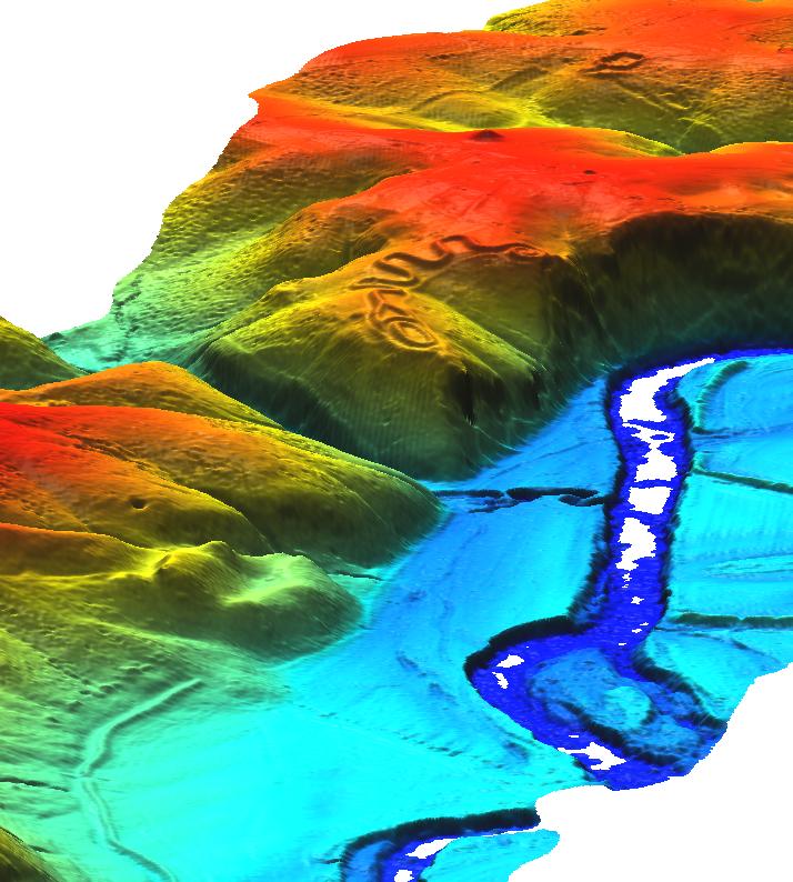
• Set the height to 500.0, the perspective to 15.0, and drag the view-puck to the North-West and reasonably zoomed in.

You should now be able to see the serpent!

The Great Serpent Mound, Adams County, Ohio, USA

Sample data

Widely used in GRASS tutorials

• Jockey's Ridge, NC, LIDAR dataset
• North Carolina OSGeo Edu data set (includes multi-return LIDAR data)

Other

• United States Antarctic Resource Center: LIDAR High-resolution DEM Final DATA Downloads
  http://usarc.usgs.gov/lidar_dload.shtml

• LIDAR ALSM Research, Arizona State University Ative Tectonics, Research Group
  http://lidar.asu.edu/research.html and http://www.geongrid.org/science/lidar.html

• USGS Center for LIDAR Information Coordination and Knowledge (aka CLICK) - USGS LiDAR point cloud distribution site
  http://lidar.cr.usgs.gov

• Washington State Geospatial Data Archive, Mount Saint Helens - Lidar Data
  https://wagda.lib.washington.edu/data/type/elevation/lidar/st_helens/

• Puget Sound Lidar Consortium, public-domain high-resolution topography for western Washington
  http://pugetsoundlidar.ess.washington.edu/index.htm

• NOAA Topographic Change Mapping LIDAR Data Retrieval Tool (LDART) NOAA Coastal Services Center
  http://maps.csc.noaa.gov/TCM/

• Landmap, LIDAR Data from the Environment Agency
  http://www.landmap.ac.uk/lidar/lidar.html

• Northern California LIDAR data
  http://quake.usgs.gov/research/geology/lidar/ and http://core2.gsfc.nasa.gov/lidar/terrapoint/

• IDAHO GEOSPATIAL , Bare Earth LIDAR DEM Download - UTM
  http://inside.uidaho.edu/geodata/LiDAR/LiDARBareEarthDEM_DownloadUTM.htm

• EarthScope Spatial Data Explorer - A java application for querying, browsing, and acquiring data from the EarthScope Spatial Data Repository. Currently includes a number of LiDAR datasets.
  http://www.earthscope.org/data/lidar.php

• LIDAR Galley
  https://peoiewswebinfo.monmouth.army.mil/JPSD/LIDAR_Gallery.htm

• South Tyrol - Download of DTMs (Homepage in German or Italian)
  http://www.provinz.bz.it/raumordnung/grundkarten/utm/default_d.htm

Links

• libLAS - LAS 1.0/1.1 ASPRS LiDAR data translation toolset