LIDAR
LIDAR and Multi-beam Swath bathymetry data
Modules
Import
- r.in.xyz - Create a raster map from an assemblage of many coordinates using univariate statistics.
(example)
- v.in.ascii - Import data from an ASCII file to GRASS vector format.
Limited to a few million data points unless topology and database creation is skipped with the -bt flags
Analysis
- v.outlier - Removes outliers from vector point data.
- v.lidar.edgedetection - Detect the object's edges from a LIDAR data set.
- v.lidar.growing - Building contour determination and Region Growing algorithm for determining the building inside.
- v.lidar.correction - Correction of the v.lidar.growing output. It is the last of the three algorithms for LIDAR filtering.
Surface generation
- v.surf.rst - Spatial approximation and topographic analysis using regularized spline with tension.
- v.surf.idw - Surface interpolation from vector point data by Inverse Distance Squared Weighting.
- v.surf.bspline - Surface interpolation from vector point data by bicubic or bilineal interpolation with Tykhonov regularization.
- r.fillnulls - Fills no-data areas in raster maps using v.surf.rst splines interpolation.
Swath Bathymetry Tools
see also the Marine_Science#Multibeam_sonar_processing wiki page
- The v.swathwidith module by David Finlayson for planning surveys. (development page)
- An example of post-processing scanned paper sidescan swaths using thin plate spline warping with GDAL's "gdalwarp -tps" function. (debugging page)
- GRASS integration with MB-System (GPL) software for processing Multibeam and Sidescan Sonar data. GRASS + MBsys + GMT make a nice scriptable trio.
LIDAR Tools
- r.terraflow - computation of flow direction, flow accumulation and other basic topographic terrain indices from massive raster digital elevation models (DEM). From the Duke University STREAM project.
- Flood simulation using r.lake. Includes fancy NVIZ visualization of Trento, Italy, by Markus Neteler.
- LAStools are a set of simple command line tools (including source code) for converting to/from ASCII, viewing, comparing, and compressing LIDAR data.
- libLAS ASPRS LiDAR data translation tools
Example
Import
- Using libLAS to import LAS data into GRASS. (data used in this example can be found at appliedimagery.com)
Import to raster DEM
Check bounds and SRS:
lasinfo "Serpent_Mound_Model_LAS_Data.las"
[...]
 Min X Y Z                  289020.900000 4320942.610000 166.780000
 Max X Y Z                  290106.020000 4323641.570000 215.480000
Spatial Reference           +proj=utm +zone=17 +ellps=WGS84 +units=m
After creating a suitable UTM zone 17 location (EPSG:32617) set the region according to the information from lasinfo at 1m resolution, rounding grid outwards to align to whole meters:
g.region n=4323641.57 s=4320942.61 w=289020.90 e=290106.02 res=1 -ap
Finally, import with r.in.xyz with data piped directly from the las2txt program and set a nice equalized color table:
BASEMAP="Serpent_Mound_Model_LAS"
las2txt --stdout "${BASEMAP}_Data.las" | \
   r.in.xyz in=- out=${BASEMAP}_Data fs=space
r.colors ${BASEMAP}_Data color=bcyr -e
Import as vector points
Region setting (establishing the grid) is not needed for vector features so we can go directly to the import step. To deal with millions of input points v.in.ascii should be run with the options to skip creation of an attribute database and building topology as these can consume large amounts of memory. Typically it is more efficient to work with huge datasets in GRASS as raster data.
las2txt --stdout "${BASEMAP}_Data.las" | \
  v.in.ascii -tbz z=3 out="${BASEMAP}_pts" fs=space

# display
d.vect "${BASEMAP}_pts" -z
After import as points you can then use the v.lidar tools to clean the data: v.lidar.correction, v.lidar.edgedetection, v.lidar.growing, and v.surf.bspline.
Clean raster DEM
# convert to vector points
r.to.vect -z feature=point in=${BASEMAP}_Data out=${BASEMAP}_pt

# interpolate using a regularized spline fit
# this is very slow, but produces very high quality output
#   r.fillnulls may be faster?
v.surf.rst layer=0 in=${BASEMAP}_pt elev=${BASEMAP}.rst

# create 5m buffer area around origial data points
r.buffer in=${BASEMAP}_Data out=${BASEMAP}.5m_buff dist=5

# crop interpolated DEM to only include areas nearby actual data
r.mapcalc "${BASEMAP}.filled = \
   if( isnull(${BASEMAP}.5m_buff), null(), ${BASEMAP}.rst)"

# set colors to something nice
r.colors ${BASEMAP}.filled color=bcyr -e
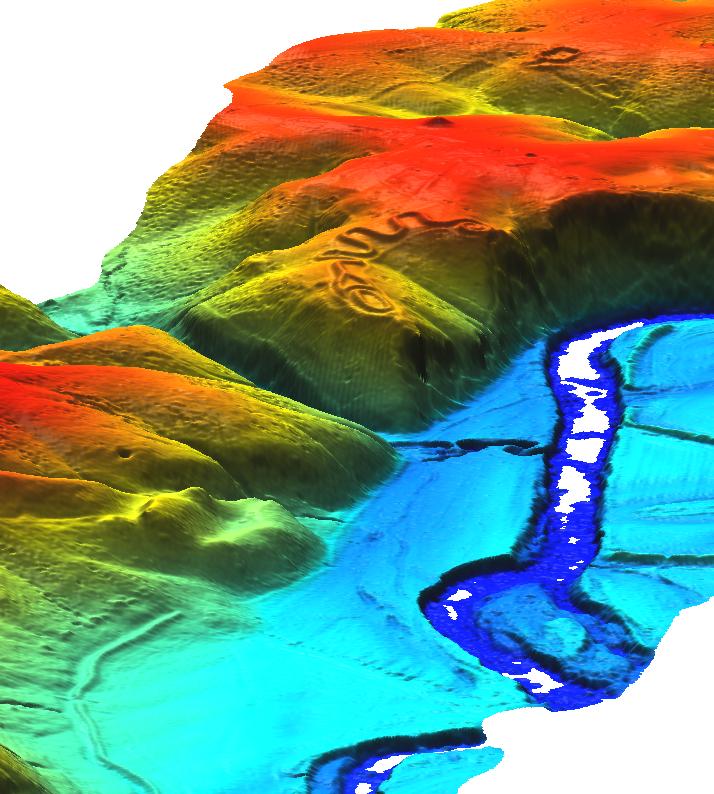
Visualize raster DEM in 3D
nviz ${BASEMAP}.filled
- Set z-exag to 2.0
- In Visualize → Raster Surfaces set the fine resolution to 1
- Set the height to 500.0, the perspective to 15.0, and drag the view-puck to the North-West and reasonably zoomed in.
- You should now be able to see the serpent!

It is possible to show vector points in 3D, but millions of them may make the program run slow. (untested)
Export
Export vector points to LAS
This is the reverse of the import step, but using v.out.ascii or r.out.xyz with txt2las. Because the v.out.ascii module exports category number which we are not interested in, we cut it away with the UNIX cut utility.
v.out.ascii ${BASEMAP}_pts fs=space | \
   cut -f1-3 -d' ' > ${BASEMAP}_export.txt
txt2las --parse xyz -i ${BASEMAP}_export.txt
Sample data
Widely used in GRASS tutorials
- Jockey's Ridge, NC, LIDAR dataset
- North Carolina OSGeo Edu data set (includes multi-return LIDAR data)
Other
- United States Antarctic Resource Center: LIDAR High-resolution DEM Final DATA Downloads
http://usarc.usgs.gov/lidar_dload.shtml
- LIDAR ALSM Research, Arizona State University Ative Tectonics, Research Group
http://lidar.asu.edu/research.html and http://www.geongrid.org/science/lidar.html
- USGS Center for LIDAR Information Coordination and Knowledge (aka CLICK) - USGS LiDAR point cloud distribution site
http://lidar.cr.usgs.gov
- Washington State Geospatial Data Archive, Mount Saint Helens - Lidar Data
https://wagda.lib.washington.edu/data/type/elevation/lidar/st_helens/
- Puget Sound Lidar Consortium, public-domain high-resolution topography for western Washington
http://pugetsoundlidar.ess.washington.edu/index.htm
- NOAA Topographic Change Mapping LIDAR Data Retrieval Tool (LDART) NOAA Coastal Services Center
http://maps.csc.noaa.gov/TCM/
- Landmap, LIDAR Data from the Environment Agency
http://www.landmap.ac.uk/lidar/lidar.html
- Northern California LIDAR data
http://quake.usgs.gov/research/geology/lidar/ and http://core2.gsfc.nasa.gov/lidar/terrapoint/
- IDAHO GEOSPATIAL , Bare Earth LIDAR DEM Download - UTM
http://inside.uidaho.edu/geodata/LiDAR/LiDARBareEarthDEM_DownloadUTM.htm
- EarthScope Spatial Data Explorer - A java application for querying, browsing, and acquiring data from the EarthScope Spatial Data Repository. Currently includes a number of LiDAR datasets.
http://www.earthscope.org/data/lidar.php
- South Tyrol - Download of DTMs (Homepage in German or Italian)
http://www.provinz.bz.it/raumordnung/grundkarten/utm/default_d.htm
Links
- libLAS - LAS 1.0/1.1 ASPRS LiDAR data translation toolset