R statistics/rgrass: Difference between revisions
Veroandreo (talk | contribs) (function updates and clean-up) |
Veroandreo (talk | contribs) (update examples to terra - wip) |
||
| Line 146: | Line 146: | ||
ncdata | ncdata | ||
class : SpatRaster | class : SpatRaster | ||
dimensions : | dimensions : 450, 500, 2 (nrow, ncol, nlyr) | ||
resolution : | resolution : 30, 30 (x, y) | ||
extent : | extent : 630000, 645000, 215000, 228500 (xmin, xmax, ymin, ymax) | ||
coord. ref. : +proj=lcc +lat_0=33.75 +lon_0=-79 +lat_1=36.1666666666667 +lat_2=34.3333333333333 +x_0=609601.22 +y_0=0 +ellps=GRS80 +units=m +no_defs | coord. ref. : +proj=lcc +lat_0=33.75 +lon_0=-79 +lat_1=36.1666666666667 +lat_2=34.3333333333333 +x_0=609601.22 +y_0=0 +ellps=GRS80 +units=m +no_defs | ||
sources : | sources : file1da12a752d65.grd | ||
file1da12112d9ea4.grd | |||
names : geology_30m, elevation | names : geology_30m, elevation | ||
min values : 217, 55. | min values : 217, 55.92321 | ||
max values : 948, 156. | max values : 948, 156.25197 | ||
</source> | </source> | ||
| Line 175: | Line 175: | ||
Min. :217.0 Min. : 56.01 | Min. :217.0 Min. : 56.01 | ||
1st Qu.:217.0 1st Qu.: 94.77 | 1st Qu.:217.0 1st Qu.: 94.77 | ||
Median :270.0 Median :108. | Median :270.0 Median :108.86 | ||
Mean :311.2 Mean :110. | Mean :311.2 Mean :110.36 | ||
3rd Qu.:270.0 3rd Qu.:126.80 | 3rd Qu.:270.0 3rd Qu.:126.80 | ||
Max. :948.0 Max. :156. | Max. :948.0 Max. :156.07 | ||
</source> | </source> | ||
| Line 211: | Line 210: | ||
=== Example 4: Summarizing data === | === Example 4: Summarizing data === | ||
<!--- this does not coincide now using the function freq in terra, so removing | |||
We can create a table of cell counts: | We can create a table of cell counts: | ||
<source lang="rsplus"> | <source lang="rsplus"> | ||
| Line 264: | Line 264: | ||
948 CZam 85 | 948 CZam 85 | ||
</pre> | </pre> | ||
---> | |||
Create a box plot of geologic types at different elevations: | Create a box plot of geologic types at different elevations: | ||
Revision as of 20:55, 19 April 2023
Installation
Terminology
See "Overview" in R_statistics
R within GRASS
In this example, we will use R within a GRASS GIS session, i.e. start R (or RStudio) from the GRASS GIS terminal or command line interface.
Startup
- First start a GRASS GIS session. Then, at the GRASS command line start R (for an 'rstudio' session, see below)
- In this example we will use the North Carolina sample dataset.
Reset the region settings to the defaults
GRASS (nc_spm_08_grass7):~ > g.region -d
Launch R from the GRASS prompt
GRASS (nc_spm_08_grass7):~ > R
Load the rgrass library:
library(rgrass)Get the GRASS environment (mapset, region, map projection, etc.); you can display the metadata for your location by printing G:
gmeta()
gisdbase    /home/mneteler/grassdata
location    nc_spm_08_grass7
mapset      user1
rows        620
columns     1630
north       320000
south       10000
west        120000
east        935000
nsres       500
ewres       500
projection:
 PROJCRS["NAD83(HARN) / North Carolina",
    BASEGEOGCRS["NAD83(HARN)",
        DATUM["NAD83 (High Accuracy Reference Network)",
            ELLIPSOID["GRS 1980",6378137,298.257222101,
                LENGTHUNIT["metre",1]]],
        PRIMEM["Greenwich",0,
            ANGLEUNIT["degree",0.0174532925199433]],
        ID["EPSG",4152]],
    CONVERSION["SPCS83 North Carolina zone (meters)",
        METHOD["Lambert Conic Conformal (2SP)",
            ID["EPSG",9802]],
        PARAMETER["Latitude of false origin",33.75,
            ANGLEUNIT["degree",0.0174532925199433],
            ID["EPSG",8821]],
        PARAMETER["Longitude of false origin",-79,
            ANGLEUNIT["degree",0.0174532925199433],
            ID["EPSG",8822]],
        PARAMETER["Latitude of 1st standard parallel",36.1666666666667,
            ANGLEUNIT["degree",0.0174532925199433],
            ID["EPSG",8823]],
        PARAMETER["Latitude of 2nd standard parallel",34.3333333333333,
            ANGLEUNIT["degree",0.0174532925199433],
            ID["EPSG",8824]],
        PARAMETER["Easting at false origin",609601.22,
            LENGTHUNIT["metre",1],
            ID["EPSG",8826]],
        PARAMETER["Northing at false origin",0,
            LENGTHUNIT["metre",1],
            ID["EPSG",8827]]],
    CS[Cartesian,2],
        AXIS["easting (X)",east,
            ORDER[1],
            LENGTHUNIT["metre",1]],
        AXIS["northing (Y)",north,
            ORDER[2],
            LENGTHUNIT["metre",1]],
    USAGE[
        SCOPE["Engineering survey, topographic mapping."],
        AREA["United States (USA) - North Carolina - counties of Alamance; Alexander; Alleghany; Anson; Ashe; Avery; Beaufort; Bertie; Bladen; Brunswick; Buncombe; Burke; Cabarrus; Caldwell; Camden; Carteret; Caswell; Catawba; Chatham; Cherokee; Chowan; Clay; Cleveland; Columbus; Craven; Cumberland; Currituck; Dare; Davidson; Davie; Duplin; Durham; Edgecombe; Forsyth; Franklin; Gaston; Gates; Graham; Granville; Greene; Guilford; Halifax; Harnett; Haywood; Henderson; Hertford; Hoke; Hyde; Iredell; Jackson; Johnston; Jones; Lee; Lenoir; Lincoln; Macon; Madison; Martin; McDowell; Mecklenburg; Mitchell; Montgomery; Moore; Nash; New Hanover; Northampton; Onslow; Orange; Pamlico; Pasquotank; Pender; Perquimans; Person; Pitt; Polk; Randolph; Richmond; Robeson; Rockingham; Rowan; Rutherford; Sampson; Scotland; Stanly; Stokes; Surry; Swain; Transylvania; Tyrrell; Union; Vance; Wake; Warren; Washington; Watauga; Wayne; Wilkes; Wilson; Yadkin; Yancey."],
        BBOX[33.83,-84.33,36.59,-75.38]],
    ID["EPSG",3358]]
Listing of existing maps
List available vector maps:
execGRASS("g.list", parameters = list(type = "vector"))List selected vector maps (wildcard):
execGRASS("g.list", parameters = list(type = "vector", pattern = "precip*"))
 precip
 precip_30ynormals
 precip_30ynormals_3d
Save selected vector maps into R vector:
my_vmaps <- execGRASS("g.list", parameters = list(type = "vector", pattern = "precip*"))
attributes(my_vmaps)
attributes(my_vmaps)$resOut
 [1] "precip"               "precip_30ynormals"    "precip_30ynormals_3d"
List available raster maps:
execGRASS("g.list", parameters = list(type = "raster"))List selected raster maps (wildcard):
execGRASS("g.list", parameters = list(type = "raster", pattern = "lsat7_2002*"))
 lsat7_2002_10
 lsat7_2002_20
 lsat7_2002_30
 lsat7_2002_40
 lsat7_2002_50
 lsat7_2002_61
 lsat7_2002_62
 lsat7_2002_70
 lsat7_2002_80
Reading in data from GRASS
Example 1: raster maps
Manual page: read_RAST()
Read in two GRASS raster maps, "geology_30m" and "elevation", from the North Carolina sample data location into the R current session as a new object "ncdata". This object is a SpatRaster layer from terra package:
ncdata <- read_RAST(c("geology_30m", "elevation"))We can verify the new R object:
ncdata
class       : SpatRaster
dimensions  : 450, 500, 2  (nrow, ncol, nlyr)
resolution  : 30, 30  (x, y)
extent      : 630000, 645000, 215000, 228500  (xmin, xmax, ymin, ymax)
coord. ref. : +proj=lcc +lat_0=33.75 +lon_0=-79 +lat_1=36.1666666666667 +lat_2=34.3333333333333 +x_0=609601.22 +y_0=0 +ellps=GRS80 +units=m +no_defs
sources     : file1da12a752d65.grd
              file1da12112d9ea4.grd
names       : geology_30m, elevation
min values  :         217,  55.92321
max values  :         948, 156.25197
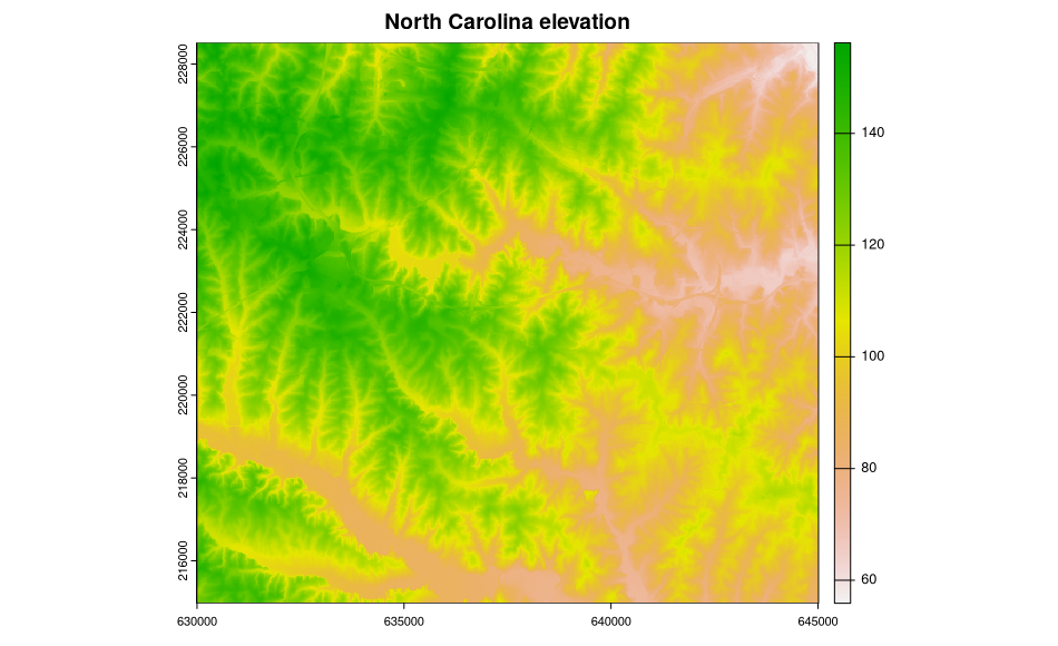
Now, let's plot one of the raster layers within the SpatRaster object. Note that we use the terra package plot function:
terra::plot(ncdata$elevation)Add a title to the plot:
title("North Carolina elevation")
In addition, we can show what is going on inside the objects read into R:
terra::summary(ncdata)
  geology_30m      elevation
 Min.   :217.0   Min.   : 56.01
 1st Qu.:217.0   1st Qu.: 94.77
 Median :270.0   Median :108.86
 Mean   :311.2   Mean   :110.36
 3rd Qu.:270.0   3rd Qu.:126.80
 Max.   :948.0   Max.   :156.07
Example 2: single raster map
Here an example for a single raster map transfer from GRASS GIS to R:
library(rgrass)
execGRASS("g.region", raster = "elevation", flags = "p")
ncdata <- read_RAST("elevation")
terra::summary(ncdata)
terra::plot(ncdata)
Example 3: vector maps
Here an example for a single vector map transfer from GRASS GIS to R. In this case, vector maps from GRASS will be converted into SpatVector objects from the terra package in R:
# needed prerequisite
library(rgrass)

execGRASS("v.info", map="schools_wake", layer="1")
vInfo("schools_wake")
myschools <- read_VECT("schools_wake")
print(terra::summary(myschools))
terra::plot(myschools)
Example 4: Summarizing data
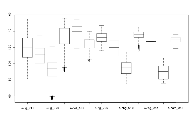
Create a box plot of geologic types at different elevations:
boxplot(ncdata$elevation ~ ncdata$geology_30m, medlwd = 1)
Example 5: Querying maps
Sometimes you may want to query GRASS GIS maps from your R session.
As an example, here the transfer of raster pixel values at the position of vector points:
# set the computational region first to the raster map:
execGRASS("g.region", raster = "elev_state_500m", flags = "p")

# query raster map at vector points, transfer result into R
goutput <- execGRASS("r.what", map="elev_state_500m", points="geodetic_pts", separator=",", intern=TRUE)
str(goutput)
chr [1:29939] "571530.81289275,265739.968425953,,187.8082200648" ...

# parse it
con <- textConnection(goutput)
go1 <- read.csv(con, header=FALSE)
str(go1)
'data.frame':	29939 obs. of  4 variables:
 $ V1: num  571531 571359 571976 572391 573011 ...
 $ V2: num  265740 265987 267049 267513 269615 ...
 $ V3: logi  NA NA NA NA NA NA ...
 $ V4: Factor w/ 22738 levels "-0.0048115728",..: 6859 6642 6749 6411 6356 6904 7506 7224 6908 7167 ...
summary(go1)
       V1               V2            V3                V4
 Min.   :121862   Min.   :  7991   Mode:logical   0      :  723
 1st Qu.:462706   1st Qu.:162508   NA's:29939     *      :  293
 Median :610328   Median :204502                  0.3048 :   47
 Mean   :588514   Mean   :200038                  0.6096 :   44
 3rd Qu.:717610   3rd Qu.:247633                  1.524  :   42
 Max.   :946743   Max.   :327186                  0.9144 :   23
                                                  (Other):28767
Exporting data back to GRASS
Finally, a SpatialGridDataFrame object is written back to a GRASS raster map:
First prepare some data: (square root of elevation)
ncdata$sqdem <- sqrt(ncdata$elevation)Export data from R back into a GRASS raster map:
writeRAST(ncdata, "sqdemNC", zcol="sqdem", ignore.stderr=TRUE)Check that it imported into GRASS ok:
execGRASS("r.info", parameters=list(map="sqdemNC"))+----------------------------------------------------------------------------+ | Map: sqdemNC Date: Sun Jul 19 13:06:34 2015 | | Mapset: PERMANENT Login of Creator: veroandreo | | Location: nc_spm_08_grass7 | | DataBase: /home/veroandreo/grassdata | | Title: ( sqdemNC ) | | Timestamp: none | |----------------------------------------------------------------------------| | | | Type of Map: raster Number of Categories: 0 | | Data Type: DCELL | | Rows: 491 | | Columns: 400 | | Total Cells: 196400 | | Projection: Lambert Conformal Conic | | N: 228500 S: 215000.0002 Res: 27.49490794 | | E: 645000 W: 630000 Res: 37.5 | | Range of data: min = 7.47818253045085 max = 12.5000787351036 | | | | Data Description: | | generated by r.in.bin | | | | Comments: | | | +----------------------------------------------------------------------------+
Using RStudio in a GRASS GIS session
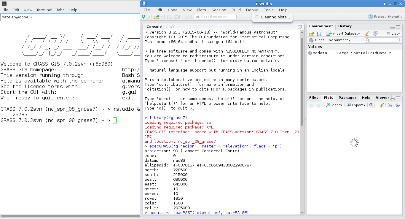
If you are most used to run R through RStudio, but still want to have all GRASS data available for performing any analyses without loosing the possibility of still using GRASS command line, you can run:
GRASS> rstudio &
or, if you already are working on a certain RStudio project:
GRASS> rstudio /path/to/project/folder/ &
Then, you load rgrass library in your RStudio project
library(rgrass)and you are ready to go.

GRASS within R
Using GRASS GIS within a R session, i.e. you connect to a GRASS GIS location/mapset from within R (or RStudio).
Startup
In the first place, find out the path to the GRASS GIS library. This can be easily done with the following command (still outside of R; or through a system() call inside of R):
# OSGeo4W, Linux, Mac OSX users:
grass --config path
It may report something like:
# OSGeo4W users:
C:\OSGeo4W64\apps\grass\grass

# Linux, Mac OSX users:
/usr/local/grass
To call GRASS GIS functionality from R, start R and use the initGRASS() function to define the GRASS settings. If GRASS GIS was installed through OSGeo4W, first start the OSGeo4W Shell. Note that it may start in C: or a directory where the user does not have writing permission. Before calling R or RStudio, first change to a directory where you are sure you have writing permission.
## MS-Windows users (example for an OSGeo4W 64bit installation)
# change to a directory with writing permission
C:\>d:
D:\>cd temp
D:\temp>cd testR

# start R within this directory:
D:\temp\testR>R

# to start RStudio from OSGeo4W Shell, run: "C:/Program Files/RStudio/bin/rstudio.exe"

# load rgrass package
library(rgrass)

# initialisation of GRASS in the North Carolina sample dataset
initGRASS(gisBase = "C:/OSGeo4W64/apps/grass/grass",
         gisDbase = "C:/Users/marissa/grassdata/",
         location = "nc_spm_08_grass7",
         mapset = "user1",
         SG="elevation")
Linux and Mac OSX users just need to start R or RStudio the usual way, load the rgrass package and initialize GRASS GIS with initGRASS() as shown below:
# load rgrass package
library(rgrass)
# initialisation of GRASS in the North Carolina sample dataset
initGRASS(gisBase = "/usr/local/grass",
          home = tempdir(),
          gisDbase = "/home/veroandreo/grassdata/",
          location = "nc_spm_08_grass7",
          mapset = "user1",
          SG="elevation")
Note: the optional SG parameter is a 'SpatialGrid' object to define the ‘DEFAULT_WIND’ of the temporary location.
# set computational region to default (optional)
system("g.region -dp")
# verify metadata
gmeta()

# get two raster maps into R space
ncdata <- read_RAST(c("geology_30m", "elevation"), cat=c(TRUE, FALSE))

# calculate object summaries
summary(ncdata$geology_30m)
 CZfg_217 CZlg_262 CZig_270 CZbg_405 CZve_583 CZam_720  CZg_766 CZam_862
     292       78      277      102        8        1        2       25
 CZbg_910   Km_921 CZam_946     NA's
      18        5        2  1009790
R in GRASS in batch mode
Run the following script with
R CMD BATCH batch.R
library(rgrass)
# initialisation of GRASS in the North Carolina sample dataset (example with a compiled version)
initGRASS(gisBase = "/home/veroandreo/software/grass/dist.x86_64-pc-linux-gnu",
          home = tempdir(),
          gisDbase = "/home/veroandreo/grassdata/",
          location = "nc_spm_08_grass7", mapset = "user1", SG="elevation",
          override = TRUE)
# set region to default
system("g.region -dp")
# verify
gmeta()
# read data into R
ncdata <- read_RAST(c("geology_30m", "elevation"), cat=c(TRUE, FALSE))
# summary of geology map
summary(ncdata$geology_30m)
proc.time()
The result is (shorted here):
cat batch.Rout
    R version 4.0.2 (2020-06-22) -- "Taking Off Again"
    Copyright (C) 2020 The R Foundation for Statistical Computing
    Platform: x86_64-redhat-linux-gnu (64-bit)
    ...
    > library(rgrass)
    Loading required package: XML
    GRASS GIS interface loaded with GRASS version: (GRASS not running)
    > # initialisation and the use of north carolina dataset
    > initGRASS(gisBase = "/home/veroandreo/software/grass/dist.x86_64-pc-linux-gnu", home = tempdir(),
    +           gisDbase = "/home/veroandreo/grassdata/",
    +           location = "nc_spm_08_grass7", mapset = "user1", SG="elevation",
    +           override = TRUE)
    gisdbase    /home/veroandreo/grassdata/
    location    nc_spm_08_grass7
    mapset      user1
    rows        13500
    columns     15000
    north       228500
    south       215000
    west        630000
    east        645000
    nsres       1
    ewres       1
    projection  +proj=lcc +lat_1=36.16666666666666 +lat_2=34.33333333333334
    +lat_0=33.75 +lon_0=-79 +x_0=609601.22 +y_0=0 +no_defs +a=6378137
    +rf=298.257222101 +towgs84=0.000,0.000,0.000 +type=crs +to_meter=1

    > system("g.region -dp")
    projection: 99 (Lambert Conformal Conic)
    zone:       0
    datum:      nad83
    ellipsoid:  a=6378137 es=0.006694380022900787
    north:      320000
    south:      10000
    west:       120000
    east:       935000
    nsres:      500
    ewres:      500
    rows:       620
    cols:       1630
    cells:      1010600
    > gmeta()
    gisdbase    /home/veroandreo/grassdata/
    location    nc_spm_08_grass7
    mapset      user1
    rows        620
    columns     1630
    north       320000
    south       10000
    ...
    > ncdata <- read_RAST(c("geology_30m", "elevation"), cat=c(TRUE, FALSE))
    ...
    > summary(ncdata$geology_30m)
    CZfg_217 CZlg_262 CZig_270 CZbg_405 CZve_583 CZam_720  CZg_766 CZam_862
         292       78      277      102        8        1        2       25
    CZbg_910   Km_921 CZam_946     NA's
          18        5        2  1009790
    > proc.time()
       user  system elapsed
      8.061   2.016  10.048
Troubleshooting
Running out of disk space
Linux: A common issue is that /tmp/ is used for temporary files albeit being often a small partition. To change that to a larger directory, you may add to your $HOME/.bashrc the entry:
# change TMP directory of R (note: of course also another directory than suggested here is fine)
mkdir -p $HOME/tmp
export TMP=$HOME/tmp
The drawback of this approach is that on modern Linux systems the /tmp/ is a fast RAM disk (based on tempfs) while HOME directories are often on slower spinning disks (unless you have a SSD drive). At least you no longer run out of disk space easily.