Temporal data processing: Difference between revisions
Veroandreo (talk | contribs) (add soeren's last paper) |
Veroandreo (talk | contribs) m (→See also) |
||
| Line 790: | Line 790: | ||
[[Category: Documentation]] | [[Category: Documentation]] | ||
[[Category:Temporal]] | [[Category: Tutorial]] | ||
[[Category: Temporal]] | |||
Revision as of 14:21, 22 July 2017
Introduction
TGRASS is the temporal enabled GRASS GIS. It is available from GRASS GIS 7 onwards. TGRASS is completely metadata based, i.e. it does not change any data but simply handles the organization of raster, vector, raster3D maps actually stored in a GRASS GIS mapset by registering in an additional internal database. This is done specifically for managing temporal and spatial extent including temporal topology.
Manual overview: https://grass.osgeo.org/grass72/manuals/temporalintro.html
Terminology Overview
- Space time raster datasets (strds) are designed to manage raster map time series. Modules that process strds have the naming prefix t.rast.
- Space time 3D raster datasets (str3ds) are designed to manage 3D raster map time series. Modules that process str3ds have the naming prefix t.rast3d.
- Space time vector datasets (stvds) are designed to manage vector map time series. Modules that process stvds have the naming prefix t.vect.
Workflow overview
- create an empty space time datasets: strds, str3ds, or stvds (t.create)
- register the GRASS GIS maps (t.register)
- check the generated space time datasets (t.list, t.info)
- do your analysis: t.rast.aggregate, t.info, t.rast.univar, t.vect.univar, ... so many more!
Example workflow for a Chlorophyll-a MODIS time series
The following examples are based on a series of MODIS L3 Chlorophyll-a product that is freely available at the ocean color site. So, say we download the SMI 8-day composite product at 4.6 km resolution for the period 2003-2013. That is a 506 set of images, 46 per year. Data comes as compressed HDF4 files. Chlorophyll products filenames look like this:
A20030012003008.L3m_8D_CHL_chlor_a_4km
 A: MODIS/Aqua
 2003: Year at start
 001: Julian day at start
 2003: Year at end
 008: Julian day at end
 L3m: Level 3 data, mapped (Projection: Plate carrée)
 8D: 8 day composition
 CHL: Chlorophyll a concentration product
 chlor_a: algorithm used 10^(a0 + a1*X + a2*X^2 + a3*X^3 + a4*X^4)
 4km: 4.6km pixel size (8640x4320 image, 2.5 minute resolution)
We now decompress files and check metadata
# Go to where the data is and decompress
  find -iname '*.bz2' -exec bzip2 -d {} \;
# Check file meta-data (GDAL utilities)
  gdalinfo A20030012003008.L3m_8D_CHL_chlor_a_4km
Next step is to import all 506 images into GRASS. You can use r.in.gdal or r.external for that. Note that global Cl-a images as downloaded from ocean color site are ~150 mb each (disk space issues!). Here, 3 different options:
- import global images (506 images, 150 Mb each) with r.in.gdal, resize to study area and remove global files
- set projection and extension, and resize to study area with gdal_translate, and import already resized images with r.in.gdal
- import global images (506 images, 150 Mb each) with r.external, resize to study area and remove global files, as showed next:
# define region extension
g.region -p n=-38 s=-55 w=-70 e=-56

suffix=_tmp
for map in *chlor* ; do
    r.external input=$map output=${map}${suffix} -o
    r.mapcalc expression="$map = ${map}${suffix}"
    g.remove type=raster name=${map}${suffix}
done
Once we have maps inside GRASS we can start the temporal processing. If this is the first time you'll use temporal modules, you need to run
t.connect -d
to set the default temporal GIS database connection for the current mapset. The default TGIS database of type sqlite3 is located in the PERMANENT mapset directory. Temporal GIS content from all created mapsets will be stored there.
Creating a STRDS and registering maps
Creating a STRDS
First step is to create a space time dataset by means of t.create. As an example, let us create a strds for the Chlorophyll-a (Cl-a) time series. We need to define the name and semantic type of the new space time dataset, its title and a description. By default a raster dataset is created with absolute time (Gregorian calendar). We can change that according to our needs with type and temporaltype options.
t.create type=strds temporaltype=absolute output=cla title="Chlorophyll-a concentration" \
description="MODIS L3 Chlorophyll-a concentration for Argentinian sea" semantictype=mean
Registering maps
Then, we register the maps in the strds using t.register. This module assigns time stamps to raster, 3D raster and vector maps and register them into space time datasets. Existing timestamps can be read and used by t.register. Note that this is a metadata based registration, nothing is imported into GRASS GIS since the maps are already present in the location (hence, no duplication occurs).
This module (and TGRASS in general) supports absolute time and relative time. The absolute temporal type refers to a fixed date or interval in the Gregorian calendar, while the relative temporal type refers to data without fixed time stamps (e.g., sequential maps used to calculate multi-decadal averages). Refer to the TGRASS overview slides for background.
Maps can be registered by command line argument (a list of comma separated map names) or using an input file. The start time, end time and a temporal increment can be provided either by command line or in the input file. End time and increment are mutual exclusive. Maps can be registered in several space time datasets using the same timestamp. For a more detailed explanation and examples on how to register maps in stds, see also maps registration wiki.
Start time and end time with absolute time must be provided using the format yyyy-mm-dd HH:MM:SS +HHMM. It is also supported to specify the date yyyy-mm-dd only. In case of relative time the temporal unit (years, months, days, hours, minutes or seconds) must be provided. The relative start time, end time and the increment are integers (see also t.register).
# note: with -i we create intervals (start and end time), for the given increment, and starting from start.
t.register -i type=raster input=cla maps=`g.list raster pattern="*_chlor_*" separator=comma` \
start="2003-01-01" increment="8 days"
Dealing with weekly data
While the former would have been the simplest solution, our 8-day products have a problem: in this example the last image of each year is not a product of an 8-day composition, but 4 or 5-day. Then, when using the increment parameter, dates (and consequently, intervals) are not set properly. The solution is to create a list of maps, with their respective start and end date. As the filenames contain information regarding year and DOY (day of year), we can use the following Python script to read filenames and transform DOY to calendar dates (Thanks Soeren!).
# Script to extract the input table for t.register from map names
# run in python
# modify to your needs

from os import walk
f = []
for (dirpath, dirnames, filenames) in walk("/path/to/the/maps"):
    f.extend(filenames)
    break
# to order the list
f.sort()

input_list=[]

import datetime
for map_name in f:
  start_year = int(map_name[1:5])
  start_day  = int(map_name[5:8])
  end_year   = int(map_name[8:12])
  end_day    = int(map_name[12:15])
  start = datetime.datetime(start_year, 1, 1) + datetime.timedelta(start_day - 1)
  end = datetime.datetime(int(end_year), 1, 1) + datetime.timedelta(end_day)
  map_list = map_name + '|' + str(start) + '|' + str(end)
  print map_list
  input_list.append(map_list)

print input_list

txt = '\n' .join(input_list)
f = open("input_list_cla.txt","w")
f.write(txt)
f.close()
Using the number of characters in the filenames and datetime library in Python, you can convert DOY in the filenames into start_time and end_time as in the list you need to pass to t.register. The resulting list looks like this:
 A20030012003008.L3m_8D_CHL_chlor_a_4km_arg|2003-01-01 00:00:00|2003-01-09 00:00:00
 A20030092003016.L3m_8D_CHL_chlor_a_4km_arg|2003-01-09 00:00:00|2003-01-17 00:00:00
 A20030172003024.L3m_8D_CHL_chlor_a_4km_arg|2003-01-17 00:00:00|2003-01-25 00:00:00
 ...
 A20133452013352.L3m_8D_CHL_chlor_a_4km_arg|2013-12-11 00:00:00|2013-12-19 00:00:00
 A20133532013360.L3m_8D_CHL_chlor_a_4km_arg|2013-12-19 00:00:00|2013-12-27 00:00:00
 A20133612013365.L3m_8D_CHL_chlor_a_4km_arg|2013-12-27 00:00:00|2014-01-01 00:00:00
and then, the command would be:
t.register --o type=raster input=cla file=input_list_cla.txt
As we are providing start and end time along with map names, we don't need to use the -i flag, neither set start nor increment options because that information is all there in the file.
Assign a color table
We can also set a color table for all maps in the strds with t.rast.colors:
# using a predetermined color table
t.rast.colors input=cla color=bcyr
#using your dedicated color table
t.rast.colors input=cla rules=path/to/your/color_table
Getting some basic info and statistics
We now check the space time data sets we have in our mapset with t.list:
t.list type=strds
and get information about our recently created strds. See t.info for additional uses.
t.info type=strds input=cla
 +-------------------- Space Time Raster Dataset -----------------------------+
 |                                                                            |
 +-------------------- Basic information -------------------------------------+
 | Id: ........................ cla@clorofila
 | Name: ...................... cla
 | Mapset: .................... clorofila
 | Creator: ................... veroandreo
 | Temporal type: ............. absolute
 | Creation time: ............. 2014-04-29 14:23:00.579342
 | Modification time:.......... 2014-05-12 09:15:08.917309
 | Semantic type:.............. mean
 +-------------------- Absolute time -----------------------------------------+
 | Start time:................. 2003-01-01 00:00:00
 | End time:................... 2014-01-01 00:00:00
 | Granularity:................ 1 day
 | Temporal type of maps:...... interval
 +-------------------- Spatial extent ----------------------------------------+
 | North:...................... -38.0
 | South:...................... -55.0
 | East:.. .................... -55.0
 | West:....................... -70.0
 | Top:........................ 0.0
 | Bottom:..................... 0.0
 +-------------------- Metadata information ----------------------------------+
 | Raster register table:...... raster_map_register_91ba57d5f0924f4fa0bd7176a1b39b2f
 | North-South resolution min:. 0.041667
 | North-South resolution max:. 0.041667
 | East-west resolution min:... 0.041667
 | East-west resolution max:... 0.041667
 | Minimum value min:.......... 0.02925
 | Minimum value max:.......... 0.26472
 | Maximum value min:.......... 5.2104
 | Maximum value max:.......... 99.953934
 | Aggregation type:........... None
 | Number of registered maps:.. 506
 |
 | Title:
 | Chlorophyll-a
 | Description:
 | Concentracion de Clorofila a
 | Command history:
 | # 2014-04-29 14:23:00
 | t.create type="strds" temporaltype="absolute"
 |     output="cla" title="Chlorophyll-a"
 |     description="Concentracion de Clorofila a" --o
 | # 2014-04-29 14:23:23
 | t.register --o type="rast" input="cla"
 |     file="map_list"
 |
 +----------------------------------------------------------------------------+
Now, we get univariate statistics from the non-null cells for each registered raster map of the strds. For that matter we use t.rast.univar which, by default, returns the name of the map, the start and end date of dataset and the following values: mean, minimum and maximum vale, mean_of_abs, standard deviation, variance, coeff_var, number of null cells, total number of cell.
t.rast.univar input=cla
Or, you can send the output to a text file using
t.rast.univar input=cla separator=comma output=stats_cla.csv
This file "stats_cla.csv" you can now open in a spreadsheet or statistical software for inspection and plotting.
Listing maps and selections
The module t.rast.list allows you to list registered maps of a strds and provides several options to get the list of maps that you want. For example, you can select different granules and also perform different queries by means of the where parameter. Some examples are:
t.rast.list input=cla method=gran granule="1 month"
# this will give one image every one month, 3 months, 1 year, or the granule you choose

t.rast.list input=cla order=min columns=id,name,start_time,min where="min <= '0.05'"
# this will order by minimum value all the maps in the strds that have a minimum value lower than or equal to 0.05

t.rast.list input=cla order=max columns=name,start_time,max where="max > '10.0'"
# maps ordered by maximum value in which maximum value is higher than 10.

t.rast.list input=cla where="start_time >= '2003-01' and start_time <= '2003-06'"
# all the maps in the first 6 month of the time series

t.rast.list input=cla where="strftime('%m', start_time)='01'"
# all the maps from January

t.rast.list input=cla where="strftime('%m-%d', start_time)='01-01'"
# all the maps from January, 1st

t.rast.list input=cla where="strftime('%w', start_time)='1'"
# all Mondays in the time series (Sunday is 0)
If you have monthly (instead of 8-day products) data and you want to list all January maps, then you can do:
t.rast.list input=cla_orig where="start_time=datetime(start_time, 'start of year', ' 0 month')"
Note: Do not forget to use single quotes around date, neither in t.rast.list nor in any other of the t.* modules offering the where option, because the clause will be ignored (i.e.: no selection performed) and no warning nor error will be printed.
Visualization
There are different visualization options for strds.
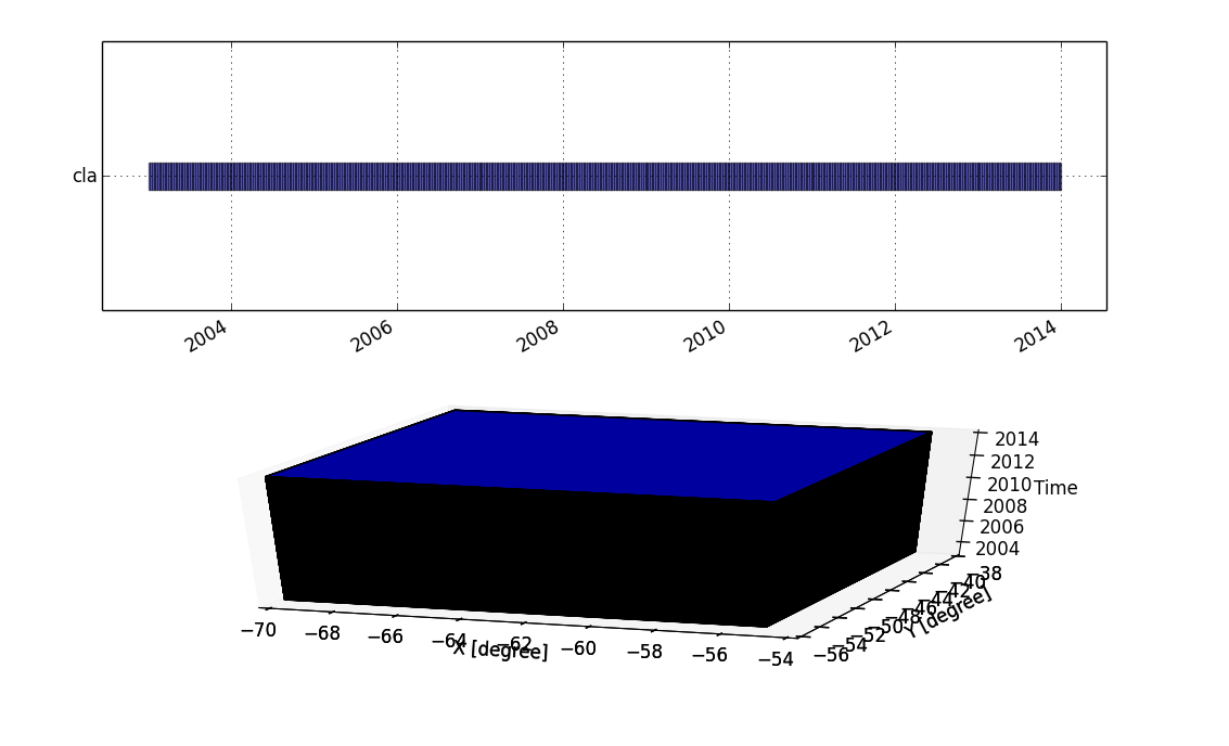
- g.gui.timeline allows to compare temporal datasets by displaying their temporal extents in a plot.
# only temporal extent
g.gui.timeline inputs=cla
# temporal and spatio-temporal extent
g.gui.timeline -3 inputs=cla
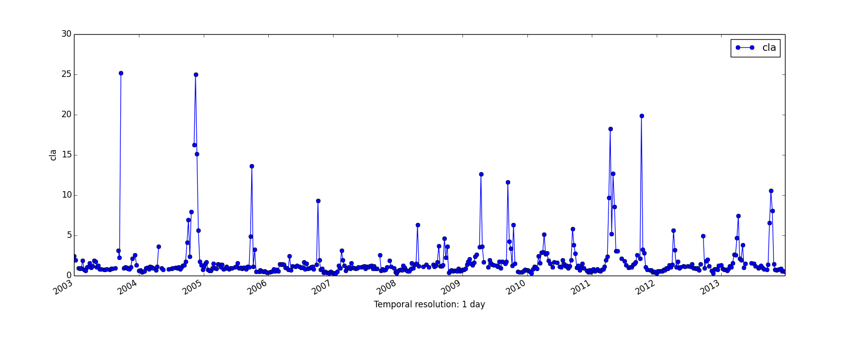
- g.gui.tplot allows to see the values of one or more temporal datasets for a queried point defined by a coordinate pair.
Steps to use this module are:
- Select strds
- Select pair of coordinates (east,north) or point in the map
- Hit Draw
- Customize plot as desired
- Save
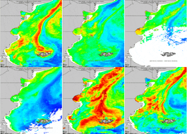
- g.gui.animation is the tool for animating a series of raster and vector maps or a space time raster or vector dataset.
g.gui.animation strds=cla_monthly_average
Aggregation
For aggregations of data with different methods and different granularities, there are two very useful commands:
- t.rast.series that performs different aggregation algorithms from r.series on all or a subset of raster maps in a strds, and
- t.rast.aggregate that temporally aggregates the maps in a strds by a user defined granularity.
With these modules it is very simple to get maps of basic statistical parameters for different temporal granules, and this permits the analysis of the spatio-temporal variability of the variable of interest.
Some examples:
# yearly aggregation
t.rast.aggregate input=cla output=cla_yearly_average basename=cla_yearly_average \
  granularity="1 years" method=average sampling=start suffix=gran

# yearly aggregation with corresponding methods (output: 7 strds with 11 maps each)
for method in average median mode minimum maximum stddev range ; do
    t.rast.aggregate input=cla output=cla_yearly_${method} \
    basename=cla_yearly_${method} granularity="1 years" \
    method=${method} sampling=start suffix=gran
done
With the where parameter, as exemplified before, we can select for example all 8-day products which start_time is 01 (January) over the years. Like this we can get the so-known climatologies.
t.rast.series input=cla method=average where="strftime('%m', start_time)='01'" output=january_average
Generalizing a bit, we can:
# monthly climatologies
for i in 01 02 03 04 05 06 07 08 09 10 11 12 ; do
  for m in average median stddev minimum maximum ; do
    t.rast.series input=cla method=${m} where="strftime('%m', start_time)='${i}'" output=${m}_${i}
  done
done

# seasonal climatologies
for i in "01 02 03" "04 05 06" "07 08 09" "10 11 12" ; do
    set -- $i ; echo $1 $2 $3
    for m in average median stddev minimum maximum ; do
        t.rast.series input=cla method=${m} output=${m}_${1} \
        where="strftime('%m',start_time)='"${1}"' or strftime('%m',start_time)='"${2}"' or strftime('%m', start_time)='"${3}"'"
    done
done
Using the climatologies previously obtained, we'll now estimate monthly anomalies in the mean, max and min Cl-a concentration. First, we need to monthly aggregate data, and then do the difference between the monthly climatology and each respective monthly aggregate. We'll do the aggregation for the average, minimum and maximum of Cl-a concentration (from 506 input maps in cla strds, we'll get 132 maps in each monthly aggregated new strds).
# monthly aggregates (132 maps)

for method in average minimum maximum ; do
    t.rast.aggregate input=cla output=cla_monthly_${method} basename=cla_monthly_${method} \
    granularity="1 months" method=${method} sampling=contains suffix=gran
done

# January anomalies in mean, min and max Cl-a

t.rast.list -s input=cla_monthly_average where="start_time=datetime(start_time, 'start of year', '0 month')" columns=name

for m in average minimum maximum ; do
    for i in 1 13 25 37 49 61 73 85 97 109 121 ; do # these numbers correspond to all january monthly aggregates
        r.mapcalc expression="Jan_${m}_anomaly_${i}=cla_monthly_${m}_${i}-01_${m}"
    done
done
You can also use t.rast.list for looping, the same way you use g.list:
for map in `t.rast.list -s input=cla_monthly_average where="strftime('%m', start_time)='01'" columns=name` ; do
    r.mapcalc expression="anomaly_${map}=${map}-01_average"
done
Generalizing, we can estimate all monthly anomalies from mean like this:
for i in `seq -w 1 12` ; do
    for map in `t.rast.list -s input=cla_monthly_average columns=name where="strftime('%m', start_time)='"${i}"'"` ; do
        r.mapcalc expression="anomaly_${map}=${map}-average_${i}"
    done
done
Say we now need to know the date of the maximum value of Cl-a concentration over all the study period and/or on a yearly basis:
# map index for the overall maximum Cl-a value
t.rast.series input=cla method=max_raster output=cla_max_index

# map index for the yearly maximum Cl-a value
t.rast.aggregate input=cla granularity="1 year" method=max_raster output=yearly_max_index basename=yearly_max_index suffix=gran
The outputs show (pixelwise) the map index in which the maximum value of Cl-a occurs (from 1 to 506 and from 1 to 46, for the whole time series and on a yearly basis, respectively). For relative time this is maybe enough, but you may then want to reclassify data to get DOY, for example. In that case, you may use r.reclass.
If you already have monthly data, you can get climatologies quite simply as follows:
# January averages
t.rast.series input=cla_monthly method=average where="start_time=datetime(start_time, 'start of year', '0 month')" output=jan_average
Spatio-temporal algebra with STRDS
The module t.rast.mapcalc allows us to perform spatio-temporal mapcalc expressions on temporally sampled maps of strds. There are spatial and temporal operators available for the "expression" string. Spatial operators, functions and internal variables are those used in r.mapcalc. Temporal internal variables supported for both relative and absolute time include: td(), start_time() and end_time(). There are also several very useful internal variables supported especially for absolute time of the current sample interval or instance, e.g.: start_doy(), start_year(), start_month() and so on (see t.rast.mapcalc manual site for further details and examples).
Some examples now. Say we did some analysis and decided that we will only consider values higher than 0.05. Then, we need to set all values below that threshold to null.
t.rast.mapcalc input=cla expression="if(cla < 0.05, null(), cla)" output=cla_corrected basename=cla_corrected
or we may also want to take negative erroneous values to the knowm minimum of the strds, so:
t.rast.series input=cla method=minimum output=min_cla
t.rast.mapcalc input=cla expression="if(cla < 0.0, min_cla, cla)" output=cla_corrected  basename=cla_corrected
We may also need to reclassify all maps in the strds according to a certain threshold, e.g.: a certain level of Cl-a that indicates bloom conditions, in order to get bloom frequency afterwards:
# reclassify
t.rast.mapcalc -n input=cla output=cla_bloom basename=cla_bloom expression="if(cla > 0.75, 1, null())"
# bloom frequency
t.rast.series input=cla_bloom output=bloom_freq method=count
Do you remember we wanted to get the DOY of maximum Cl-a value before? Well, here's another way of doing it...
# overall maximum value
t.rast.series input=cla method=maximum output=max_cla
# new strds with DOY of overall maximum
t.rast.mapcalc -n inputs=cla output=date_max_cla expression="if(cla == max_cla,start_doy(),null())" basename=date_max_cla
# map with DOY of overall maximum
t.rast.series input=date_max_cla method=maximum output=max_cla_date
# remove date_max_cla strds (we were only interested in the resulting aggregated map)
t.remove -rf inputs=date_max_cla
In the development version of GRASS GIS, there's also a t.rast.algebra module that allows for temporal and spatial operations on strds by means of temporal raster algebra. The module expects an expression as input parameter in the following form: "result = expression".
The statement structure is similar to r.mapcalc, the result is the name of a new strds that will contain the result of the calculation given as expression. Expressions can be any valid or nested combination of temporal operations and spatial overlay or buffer functions that are provided by the temporal algebra. See the manual for further details and explanations.
We'll use this module to estimate the rate of change (slope) between every pair of maps in the "cla" strds. The result will be a new strds consisting of maps with the slope value between every consecutive pair of maps in the original strds:
t.rast.algebra expression="slope_cla = (cla[1]-cla[0])/8.0" basename=slope_cla
# we set 8 as fixed denominator, because products are 8-day compositions
We can then use any of the aggregation modules that we saw before to get the maximum or minimumm rate of change for different granularities.
Some known issues with t.rast.mapcalc
It has been observed that if the names of inputs and output space time datasets (partially) match each other, t.rast.mapcalc may not work properly (especially when several input strds are used). This is because the module uses a simple search and replace approach to substitute the input STRDS with the corresponding map names. Eventualy, choosing a specific order for the input STRDS in the input parameter may reduce the risk of wrong substitution. Therefore, especially in operations involving several STRDS (with partially matching names) as inputs, it might be better to use t.rast.algebra that correctly recognizes spatio-temporal datasets. However, t.rast.algebra is still experimental and only available in development version.
Subseting and something else
t.rast.extract is another really useful module in temporal GRASS. It allows to extract a subset of a strds and store it in a different strds. You use the "where" condition to do the subset, but you can also specify a r.mapcalc sub-expression that performs operations on all maps of the selected subset. If no r.mapcalc expression is defined, the selected maps are simply registered in the new output strds.
Say we need to need to know in how many maps of the strds min values are below a threshold, and not only that, but you also want to know how many pixels per map meet that condition. Then, we can do
t.rast.extract input=cla where="min <= '0.05'" output=cla_less_05 basename=cla_less_05 expression="if(cla<0.05,1,null())"
to extract those maps with a minimum value lower than 0.05, and in the same step put 1 in every cell meeting the criterium and null everywhere else. To get a count of maps and pixels meeting the condition we may use:
# univariate stistics to get the count per map
t.rast.univar input=cla_less_05
# count map of cells with min value < 0.05
t.rast.series input=cla_less_05 output=count_cla_less_05 method=count
Importing / Exporting strds
Say we now need to do some processing in R (e.g.: run DINEOF to fill gaps in data), so we need to export our strds, hence we use t.rast.export.
t.rast.export input=cla output=cla4R compression=gzip
After we have done our analysis we can import the whole strds back to GRASS again, exporting it from R with read/write.tgrass from spacetime R package and using t.rast.import in GRASS.
t.rast.import input=cla_from_R.tar.gz output=cla_from_R basename=new_map directory=/tmp
For a full example of how to handle raster time series between GRASS and R, please visit the time series GRASS-R Statistics wiki. The example is based on North Carolina climate location [1] and includes the following steps:
- Exporting the strds out of GRASS
- Importing into R
- Re-formating the data
- Running DINEOF
- Re-constructing the raster time series
- Exporting out of R, and
- Importing the gap-filled new strds into GRASS.
Neighborhood analysis
t.rast.neighbors performs a neighborhood analysis for each map in a space time raster dataset. This module supports a subset of the options already available in r.neighbors. Both, size of the neighborhood and aggregation method can be chosen. As an example, we'll estimate mean Cl-a concentration in a 3x3 neighborhood for every map in the strds.
t.rast.neighbors input=cla output=cla_smoth base=cla_smooth method=average size=3
Filling and reconstructing time series data with gaps
Harmonic ANalysis of Time Series - HANTS
r.hants is an add-on not strictly within the temporal modules, but really useful when working with this kind of data, particularly with gappy data. Here's a simple example for generating a list of temporally ordered maps to use as input in r.hants, running HANTS and getting a map of dominant frequencies, afterwards. See the manual for further information on parameter setting and explanations.
# use t.rast.list to create a list of temporally ordered maps
t.rast.list input=cla order=start_time columns=name -u > map_list.csv

# a HANTS run using the list of maps
r.hants -l file=map_list.csv nf=5 fet=0.1 dod=11 base_period=46 suffix=_hants amplitude=amp_hants phase=pha_hants

# dominant frequency map (0 means the dominant freq is 1, 1 that dominant freq is 2, and so on...)
r.series input=`g.list raster pattern=amp_hants* separator=comma` output=dominant_freq_hants method=max_raster
Local Weighted Regression - LWR
Another very useful add-on for the reconstruction of gappy time series, such as those from remote sensing imagery, is r.series.lwr. This module performs a local weighted regression (LWR) of the input time series of maps in order to estimate missing values and identify (and remove) outliers. See the manual for further information and explanations.
# use same list as before
t.rast.list input=cla order=start_time columns=name -u > map_list.csv

# run r.series.lwr
r.series.lwr file=map_list.csv suffix=_lwr order=2 weight=tricube range=0.0,65.0 dod=16 fet=0.1 -l
Estimate Mean Absolute Error (MAE)
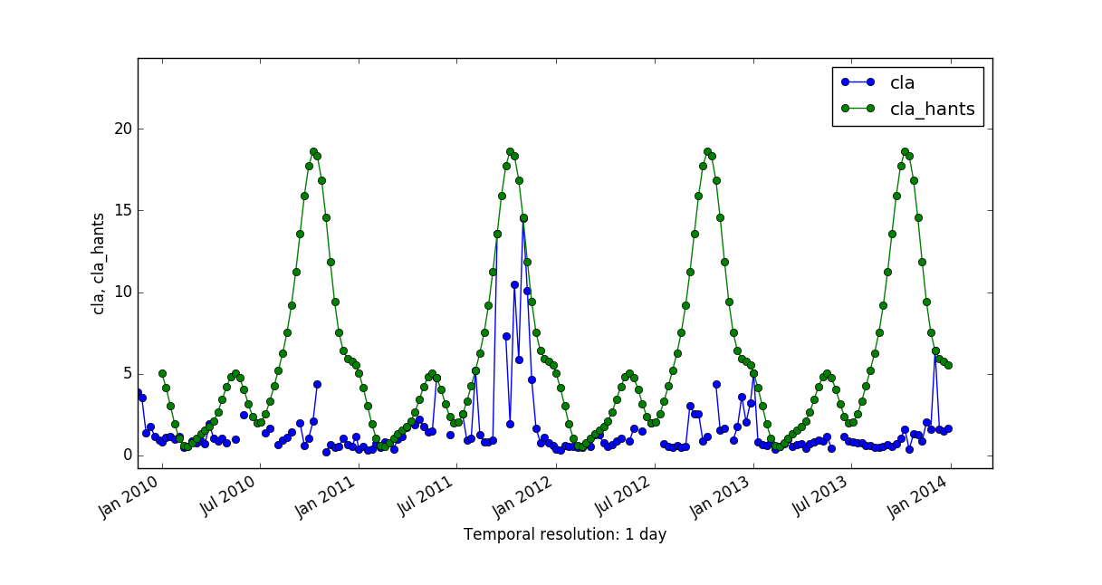
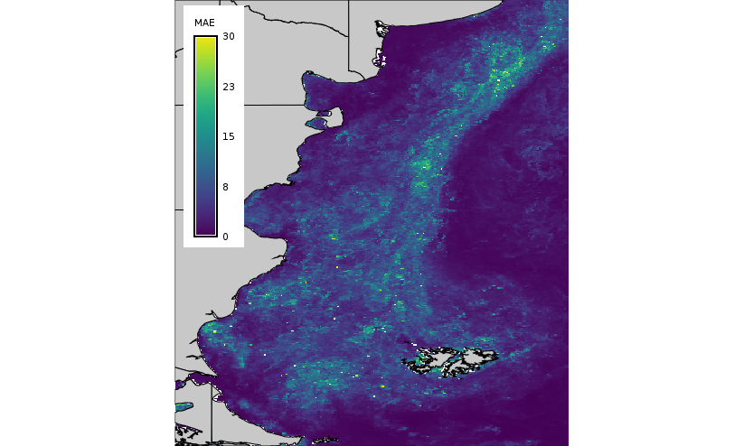
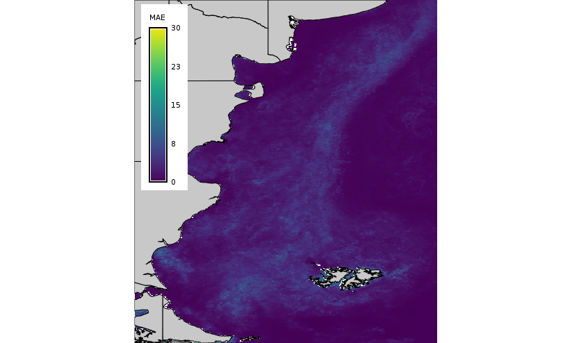
One of the measures used to assess how close forecasts or predictions might be to the observed values is the mean absolute error. We will use it to evaluate the performance of HANTS and LWR.
First, we will rebuild our time series with the corresponding output maps of r.hants and r.series.lwr. Here, only showed for LWR.
# re-build time series
t.create type=strds temporaltype=absolute output=cla_lwr \
 title="LWR output for Chl-a" \
 description="MODIS Aqua L3 Chl-a 8-day 4km 2010-2013. Reconstruction with r.series.lwr"

# create list with filenames to parse
g.list type=raster pattern="*lwr" output=names_list

# parse filenames, convert YYYY-DOY to YYYY-MM-DD and write file to use in t.register
for mapname in `cat names_list` ; do
  year_start=`echo ${mapname:1:4}`
  doy_start=`echo ${mapname:5:3}`
  year_end=`echo ${mapname:8:4}`
  doy_end=`echo ${mapname:12:3}`
  # convert YYYY-DOY to YYYY-MM-DD
  #BEWARE: leading zeros make bash assume the number is in base 8 system, not base 10!
  doy_start=`echo "$doy_start" | sed 's/^0*//'`
  doy_end=`echo "$doy_end" | sed 's/^0*//'`
  START_DATE=`date -d "${year_start}-01-01 +$(( ${doy_start} - 1 ))days" +%Y-%m-%d`
  END_DATE=`date -d "${year_end}-01-01 +$(( ${doy_end} ))days" +%Y-%m-%d`
  # print mapname, start and end date
  echo "$mapname|$START_DATE|$END_DATE" >> map_list_start_and_end_time.txt
done

# register maps in strds
t.register input=cla_lwr type=raster file=map_list_start_and_end_time.txt
Now, we will estimate the MAE and use it to compare both methods. Again, only the example for LWR is showed.
# obtain a strds of the absolute differences between predicted and observed Chl-a values
t.rast.algebra -n basename=lwr_minus_orig \
expression="abs_lwr_minus_orig = abs(cla_lwr - cla)"

# sum of the absolute differences (numerator) and count of non-null maps per pixel (denominator)
t.rast.series input=abs_lwr_minus_orig output=sum_abs_lwr_minus_orig method=sum
t.rast.series input=abs_lwr_minus_orig output=count_abs_lwr_minus_orig method=count

# MAE for LWR
r.mapcalc expression="mae_lwr = sum_abs_lwr_minus_orig / count_abs_lwr_minus_orig"

# remove intermediate strds and maps
t.remove -rf abs_lwr_minus_orig
g.remove -f type=raster name=sum_abs_lwr_minus_orig,count_abs_lwr_minus_orig
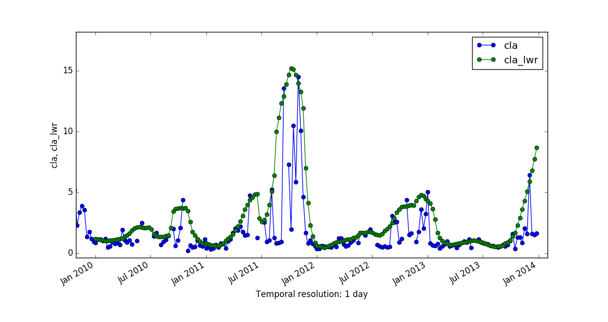
Let's now compare the predictions generated by both methods, HANTS and LWR, and the corresponding mean absolute error maps.
 |
 |
 |
 |
Extract strds values for points in a vector
Let's say we need to extract values of the strds to check the behaviour of HANTS at given locations and compare it with the original values, you can graphically do that with g.gui.tplot. But, if you need to take data outside GRASS, say, read it into R and do some other analysis (See R_Statistics wiki page) you may use v.what.strds. This module retrieves raster values from a given strds to the attribute table of a point vector map.
# original data
v.what.strds --overwrite input=points_cla strds=cla output=points_cla_out
v.db.select map=points_cla_out file=ts_points_cla.csv

# HANTS' reconstructed data (several runs)
for i in `seq 1 13` ; do
    v.what.strds --overwrite input=points_cla strds=cla_hants_${i} output=points_hants_${i}_out
    v.db.select map=points_cla file=ts_points_hants_${i}.csv
done
Another option would be to use t.rast.what that samples a space time raster dataset at specific vector point coordinates and write the output to stdout or text file using different layouts. You don't write the vector's attribute table in this case.
t.rast.what points=points strds=cla output=cla_points.csv null_value=NA separator=comma
TODO
(add some more)
FAQ
Best practice data organization
When it come to time series, often thousands of maps are involved. In order to keep control, here some suggestion
- separate original data from derived aggregates: store them in separate mapsets
- for specific projects, maintain them in individual mapsets. You can access the STDS stored in other mapsets (same location) through
t.some.module input=my_strds@the_other_mapset output=result ...
as long as mapsets are indeed accessible, i.e.: in the mapset's search path (See g.mapsets).
Best practice multi user management
GRASS GIS supports multi-user data management and offers the possibility that several users work in the same location within their own mapsets. Data can be read from other mapsets but not edited there. The same principle applies to space time datasets (STDS), i.e. in case of having a collection of maps corresponding to a time series in a dedicated mapset, you need to also create the STDS therein (See t.create and t.register), so it is visible to other users in other mapsets when they use t.list, for example.
Use of where parameter (from ticket #2270)
Pay attention when using the "where" option in t.* modules. In some occasions it may not yield the expected results. Given the backend database chosen for TGRASS implementation, you may not be selecting all maps you think if you forget to set time along with date in the where clause. For example, let's say we need to select maps from 2005-03-01 until 2005-05-31 included. You would think the following command would do the job:
t.rast.list daily_temp where="start_time > '2005-03-01' and start_time <= '2005-05-31'"
but, no... The last map in the list is:
temp_0516|pruebas|2005-05-30 00:00:00|2005-05-31 00:00:00
which would be equivalent to:
t.rast.list daily_temp where="start_time > '2005-03-01' and start_time < '2005-05-31'"
This is a product of sqlite. Therefore, if you need the last date included in your selection (map from 2005-05-31 in our example), you need to set time too.
t.rast.list daily_temp where="start_time > '2005-03-01' and start_time <= '2005-05-31 00:00:00'" | tail -n1
temp_0517|pruebas|2005-05-31 00:00:00|2005-06-01 00:00:00
Aggregation with defined granularity
Q: I need to aggregate a strds with a granularity of 1 year, but shifting the start day one month in each run, i.e.: changing the start_time to 2003-02-01, 2003-03-01, 2003-04-01 and so on... My question is: if i recursively change start_time with the 'where' parameter, will the module t.rast.aggregate "aggregate" to the next february, march, april (what i'd wish) or just till the end of 2003?
A: If you specify a granularity of a year, then the start time to perform the aggregation will always be shifted to the 1st January of the current year and the end time the 1st January of the next year (eg. 2002-01-01 - 2003-01-01). If you wish to aggregate a full year but shifting one month forward then simply use a granularity of 12 months.
Listing maps with specific start month
Q: I have a strds with 506 maps that correspond to 8-day composite products. I need to sequentially list all maps which "start_month" is January, February and so on... to use them as input in r.series (or {{cmd|t.rast.series}). How can I achieve that?
A: You can use the datetime functionality of SQLite to perform this task, this should work for January:
t.rast.list input=cla_null_mayor65 \
where='start_time >= datetime(start_time, "start of year") and start_time <= datetime(start_time, "start of year", "1 month")'
Aggregation of seasonal data
Q: How can I calculate average seasonal temperature starting from a daily temperatures temporal dataset?
A: Use t.rast.aggregate.ds, the input is the daily strds, the sampling stds should have seasonal intervals. Then use average as method. The output will have seasonal aggregated temperatures. For a detailed workflow see: seasonal aggregation example.
Aggregation of seasonal data using time ranges
A way to aggregate seasons from daily data without granularity but by using time ranges is shown here. The issue is to include for the season calculation also a month from the previous year. This can be addressed by some datetime calculations in SQLite:
# We assume to have daily temperature data in DB "temp_daily_average"

# loop over seasons, generate aggregates:
### 'start_time' and 'end_time' are columns in TGRASS

for year in `seq 2004 2014` ; do

    # we consider also a month of the previous year
    for month in "12 01 02" "03 04 05" "06 07 08" "09 10 11" ; do
        set -- $month ; echo $1 $2 $3

        prevyear=$year
        if [ $1 -eq 12 ] ; then
           prevyear=`expr $year - 1`
        fi

        # prepare query strings in SQLite
        MYSTART=`echo "SELECT strftime(datetime('${prevyear}-${1}-01'));" | sqlite3`
        MYEND=`echo "SELECT strftime(datetime('${prevyear}-${1}-01','+3 month'));" | sqlite3`

        # Debugging only, to see what it does:
        echo "---- Querying ${prevyear}-${1}-01 ... ${year}-${3}-end:"
        # we use start_time and end_time to get the proper time range
        t.rast.list input=temp_daily_average@modis_lst_reconstructed_europe_daily \
        where="start_time >= '$MYSTART' AND end_time <= '$MYEND'" > list_${prevyear}_${1}_${3}.csv

        head -n 3 list_${prevyear}_${1}_${3}.csv
        echo "..."
        tail -n 3 list_${prevyear}_${1}_${3}.csv
        echo "======="
        rm -f list_${prevyear}_${1}_${3}.csv

        # calculate aggregates:
        method="average"   # median mode minimum maximum stddev

        t.rast.series input=temp_daily_average@modis_lst_reconstructed_europe_daily \
        where="start_time >= '$MYSTART' AND end_time <= '$MYEND'" \
        output=temp_${method}_${prevyear}_${1}
    done
done
Much simpler alternative (which runs in parallel on multi-cores):
t.rast.aggregate input=A output=B basename=b where="start_time >= '2004-03-01 00:00:00'" granularity="3 months"
Online tutorials and courses
- The temporal GRASS GIS framework: Introduction and application by Sören Gebbert (2012)
- Spatio-temporal data handling and visualization in GRASS GIS - FOSS4G 2014 workshop by Vaclav Petras, Anna Petrasova, Helena Mitasova, Markus Neteler (2014)
- Processing ERA-Interim dataset in netcdf using GDAL and GRASS GIS by Sajid Pareeth (2015)
- CZ: Úvod do časoprostorových analýz (Introduction to space-time analysis) by Martin Landa (2015)
References
- Gebbert, S., Pebesma, E. 2014. TGRASS: A temporal GIS for field based environmental modeling. Environmental Modelling & Software 53, 1-12 (DOI) - preprint PDF
- Gebbert, S., Pebesma, E. 2017. The GRASS GIS temporal framework. International Journal of Geographical Information Science 31, 1273-1292 (DOI)
See also
- Introduction: GRASS as a Temporal GIS by Sören Gebbert (slides)
- The temporal GRASS GIS framework: Introduction and application Video of Sören Gebbert's presentation in GEOSTAT course 2012
- Introduction to temporal modules (GRASS GIS manual)
- Available temporal modules (GRASS GIS manual)
- Temporal Extension (background info in trac)
- GRASS GSoC 2013 Temporal GIS Algebra for raster and vector data in GRASS