R.sun
Help page
- r.sun manual page
Tips
The speed of r.sun may be improved if r.horizon is used first and the resulting maps are given as input to r.sun. Background: the horizon needs to be computed only one time before, not in every step within r.sun. See the example at the end of the r.sun help page.
- Counterpoint: modern CPUs are fast enough that the time it takes to read the horizon map off the hard drive may be more than just calculating the horizon on-the-fly, with the added advantage that the on-the-fly horizon is always at exactly the right azimuth. You will need to test to see if r.horizon is better or worse for your own use case.
The aspin and slopein maps are needed if you wish to include the effect of reflected light (seen in both the refl_rad and global radiation output maps). These two maps can be generated from your DEM or DSM with the r.slope.aspect module.
The latin and longin maps are generally only needed if you are running r.sun from a simple XY location. In normal use with a known map projection they are not needed.
If you are in a coastal area you can speed up processing by setting regions of water to NULL in the DEM input raster map. See the r.null module. Note that this may reduce the amount of reflected light in the global and refl_rad output maps. I suspect that r.sun does not model glint off water at low sun angles, although you may have luck setting water masses to a high albedo with the albedo input raster if that is important to you.
Testing
Create an artificial surface containing a Gaussian mound:
r.surf.volcano out=gauss method=gaussian kurtosis=1
Overlay some 200m contours to show underlying topography:
r.contour in=gauss out=gauss_200m_contours step=200
d.vect gauss_200m_contours color=white
Set map's color table to highlight detail:
r.colors rad_test.day355.beam col=bcyr -e
d.legend rad_test.day355.beam range=1300,1500
Time step
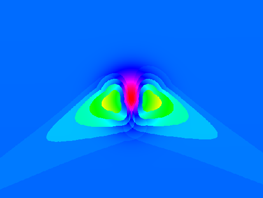
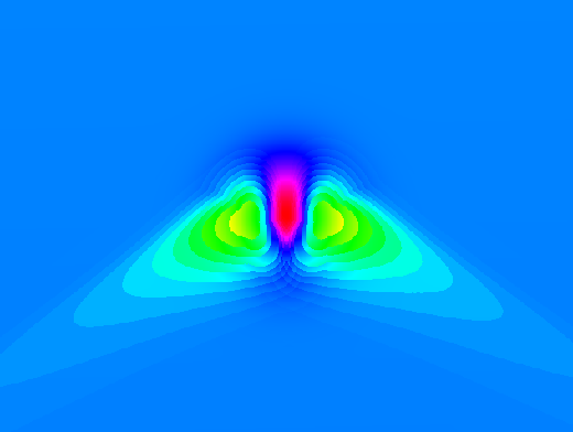
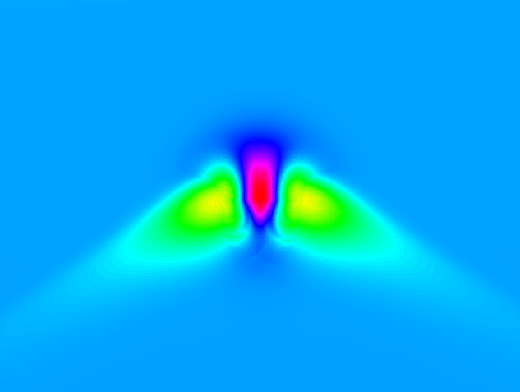
The following three images demonstrate the effects of using different time step parameters.
- step is measured in decimal hours
r.sun -s elevin="gauss" glob_rad="rad.global.30minT" day=180 step=0.5

r.sun -s elevin="gauss" glob_rad="rad.global.15minT" day=180 step=0.25

r.sun -s elevin="gauss" glob_rad="rad.global.03minT" day=180 step=0.05

The 3 minute time step takes roughly ten times as long to run as the 30 minute timestep.
Optional input maps
Using both input aspect and slope maps (generated from the input DEM) are necessary if you wish to include the effect of reflected light in the global output map.
- aspin= and slopein= options: create slope and aspect maps with the r.slope.aspect module.
- Caution: potentially buggy. See trac #498.
Using horizon seed maps can (?, unclear) speed up processing. This is especially important if you will batch process e.g. for every day of the year.
- horizon= and horizonstep= options: Pre-calculate horizon shadows by creating a series of horizon rasters with the r.horizon module.
- Results may not be as smooth as without using this option?? See trac #498.
- Estimated speedup: ?%. Depends on the number of horizon maps. Note for accuracy you might want a large number of pre-calculated horizon maps, but that comes with the downside of it taking a long time and lots of memory to load them off the disk. Calculating horizons in real-time in the CPU may in fact be both more accurate and faster. More tests are needed to clarify this issue.
- latin= and longin= options: Pre-calculate latitudes and longitudes for each raster cell. This is only needed if you are running r.sun in a simple XY location. If you are running in a normal session with a known map projection the lat/lon are calculated on the fly.
- The following script will create a raster containing latitude as the raster value:
 # create latitude map (WGS84)
 g.region rast=elevation.dem
 r.mapcalc one=1
 r.out.xyz one | \
   cut -f1,2 -d'|' | \
   m.proj -oed --quiet | \
   sed -e 's/[ \t]/|/g' | \
   cut -f1-4 -d'|' | \
   r.in.xyz in=- z=4 out=elevation.lat
 g.remove one
Creating the longitude map is exactly the same but use column 3 of the m.proj output instead of column 4:
 # create longitude map (WGS84)
 g.region rast=elevation.dem
 r.mapcalc one=1
 r.out.xyz one | \
   cut -f1,2 -d'|' | \
   m.proj -oed --quiet | \
   sed -e 's/[ \t]/|/g' | \
   cut -f1-4 -d'|' | \
   r.in.xyz in=- z=3 out=elevation.lon
 g.remove one
- Estimated speedup: 1.3% (in one test).
- See trac #498.
The above assumes that your projection's ellipsoid is WGS84. If it isn't, use other proj_out= terms with m.proj as required instead of the -o flag.
Linke turbidity factor values
- See Remund et al. (2003) appendix/table 1 for a list of monthly values for many sites around the world:
- A good description and recipe for calculating it here: (section 3.3.4, page 22)
- Download 5' global dataset for all months of 2010 as LL/WGS84 GeoTIFF here:
- https://www.soda-pro.com/help/general-knowledge/linke-turbidity-factor
- "The Linke turbidity factor (TL, for an air mass equal to 2) is a very convenient approximation to model the atmospheric absorption and scattering of the solar radiation under clear skies. It describes the optical thickness of the atmosphere due to both the absorption by the water vapor and the absorption and scattering by the aerosol particles relative to a dry and clean atmosphere. It summarizes the turbidity of the atmosphere, and hence the attenuation of the direct beam solar radiation. The larger TL, the larger the attenuation of the radiation by the clear sky atmosphere.
- The TL denotes the transparency of the cloudless atmosphere. If the sky were perfectly dry and clean, TL would be equal to 1. When the sky is deep blue, the TL is just above 1 and still very small. In summer, in Europe, the water vapour is often large and the blue sky is close to white -- the TL is larger than 3. In turbid atmosphere, e.g. in polluted cities, the TL is close to 6 - 7."
Automation
It can be tedious to set up and run a long series of r.sun simulations for every day of the year. To automate this we can write a small shell script loop:
 for DAY in `seq 1 365` ; do
    DAY_STR=`echo $DAY | awk '{printf("%.03d", $1)}'`
    echo "Processing day $DAY_STR at `date` ..."

    LINKE="`g.linke_by_day.py $DAY`"

    r.sun -s elevin=elevation.dem day=$DAY lin=$LINKE step=0.05 \
        beam_rad=rad_beam.$DAY_STR diff_rad=rad_diffuse.$DAY_STR \
        refl_rad=rad_reflected.$DAY_STR glob_rad=rad_global.$DAY_STR \
        insol_time=rad_insol_time.$DAY_STR
 done
- g.linke_by_day.py is a small program which will return the Linke coefficient for any day of the year, interpolated from monthly values. You need to edit the script to fill in values appropriate for your study area.
- If you have a multi-core CPU and you'd like to speed things up, here is a small Bourne shell script implementing a poor-man's multi-processing trick:
 ### r.sun mode 2 loop ###
 BEGIN=1
 END=365
 STEP=1
 NUM_CORES=4

 for DAY in `seq $BEGIN $STEP $END` ; do
    DAY_STR=`echo $DAY | awk '{printf("%.03d", $1)}'`
    echo "Processing day $DAY_STR at `date` ..."

    LINKE="`g.linke_by_day.py $DAY`"

    CMD="r.sun -s elevin=elevation.dem day=$DAY lin=$LINKE step=0.05 \
         beam_rad=rad_beam.$DAY_STR diff_rad=rad_diffuse.$DAY_STR \
         refl_rad=rad_reflected.$DAY_STR glob_rad=rad_global.$DAY_STR \
         insol_time=rad_insol_time.$DAY_STR --quiet"

    # poor man's multi-threading for a multi-core CPU
    MODULUS=`echo "$DAY $STEP $NUM_CORES" | awk '{print $1 % ($2 * $3)}'`
    if [ "$MODULUS" = "$STEP" ] || [ "$DAY" = "$END" ] ; then
       # stall to let the background jobs finish
       $CMD
       sleep 2
       wait
       #while [ `pgrep -c r.sun` -ne 0 ] ; do
       #   sleep 5
       #done
    else
       $CMD &
    fi
 done
 wait   # wait for background jobs to finish to avoid race conditions
- For a r.sun Mode 1 loop, see the Parallelizing Scripts page.
Minimum number of days needed to summarize a solar year
You can get an estimated curve of daily irradiation throughout the year by running r.sun for e.g. just the middle day of each month, or just for the solstices, equinoxes, and half way between them.
For example:
Day of year for minimal annual summary Day DOY Comment Feb 5th 036 mid Mar 21st 080 equinox May 6th 126 mid Jun 21st 172 solstice Aug 6th 218 mid Sept 21st 264 equinox Nov 6th 310 mid Dec 21st 355 solstice
You may want to duplicate the results from Dec. 21st as day -10 when you fit the curve in your plot.
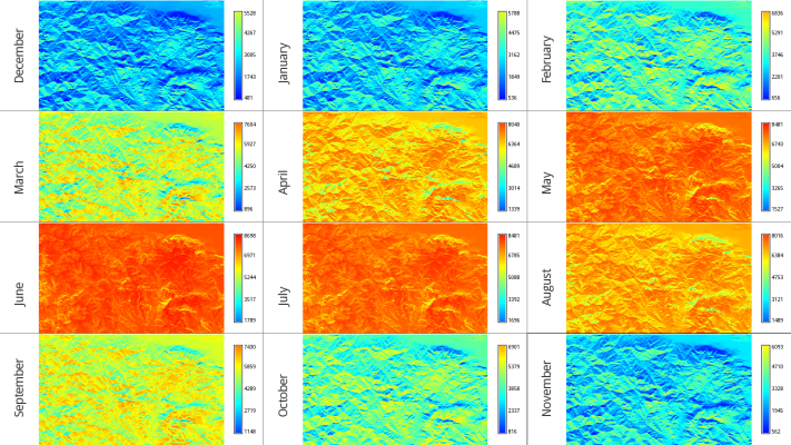
Overview of monthly maps
Given there are mean monthly global irradiation maps calculated, an overview map of all 12 maps can be drawn along with their legends (see also Common legends for many raster maps). The script assumes a common naming convention for all 12 monthly average maps (i.e. global_rad_avg.jan, global_rad_avg.feb, global_rad_avg.mar, etc.).
 #!/bash/sh
 # script to draw monthly (mean) global solar irradiation maps in a 3x4 matrix

 # set wide aspect ratio (16:9, e.g. 1366 width x 768 height)
 d.monsize setm=x0 setw=1366 seth=768

 # split in 12 frames
 d.split.frame frames=12

 # preferred font?
 d.font DroidSans

 for FRAME in "uno dec December" "dos jan January" "tres feb February" \
 "cuatro mar March" "cinco apr April" "seis may May" \
 "siete jun June" "ocho jul July" "nueve aug August" \
 "diez sep September" "once oct October" "doce nov November"

 do

    # parse "${FRAMES_STR}" and set positional parameters
    set -- $FRAME ; echo $1 $2 $3

    # select FRAME
    d.frame -s "${1}"

    # draw the map
    d.rast global_rad_avg."${2}"

    # draw label on the left and vertically
    d.text text="${3}" size=10 color=50:50:50 at=9,25 rotation=90

    # draw legend
    d.legend global_rad_avg."${2}" -s at=10,90,89,92

 done

Same image also here (a bit of higher resolution)
Development
- Ongoing trials documented in trac ticket #498
OpenCL
As part of the Google Summer of Code 2010 an OpenCL version has been written that allows r.sun to run on GPUs. This provides a massive speedup in processing time. The merging of this code into GRASS 7's r.sun is forthcoming (HB).
- To get your hands on the code now see http://github.com/mailseth/OpenCL-integration-for-GRASS---GDAL (functional prototype now available)
- To use OpenCL GPU functionality you'll want a graphics card like the ATI HD5770 or nVidia GTX260 or GTX460, or newer.
- OpenCL also allows for running on multi-core (or multi-processor) CPUs, for systems without GPUs. You can run OpenCL via multicore *or* GPU, but not both on the same job at the same time.
- Seth wrote: The OpenCL version of r.sun runs over 20x faster than the original version on my machine (2.26 GHz Mac Pro vs. GeForce GTX 285). However, it is hampered by the low memory on your GPU, so you may need to partition your raster.
- You can now ./configure GRASS 7 with OpenCL support using:
--with-opencl
ToDo
- Merge in OpenCL code
- Add support for OpenMP parallelization (if OpenCL doesn't make that redundant)
References
Usage of r.sun in the literature (selected references):
- Agugiaro, G., Remondino, F., Stevanato, G., De Filippi, R., Furlanello, C., 2011. Estimation of solar radiation on building roofs in mountainous areas. International Archives of Photogrammetry 38. PDF: http://www.pf.bv.tum.de/isprs/pia11/pub/PIA11_Agugiaro_et_al.pdf
- H.T. Nguyen and J.M. Pearce, "Estimating Potential Photovoltaic Yield with r.sun and the Open Source Geographical Resources Analysis Support System" Solar Energy 84, pp. 831-843, 2010. Open Access (see also Link to related external wiki page)
- Hofierka, J., Kanuk, J., 2009. Assessment of photovoltaic potential in urban areas using open-source solar radiation tools. Renewable Energy 34, 2206-2214.
- Huld, T.A., Šúri, M., Dunlop, E.D., Micale, F., 2006. Estimating average daytime and daily temperature profiles within Europe. Environmental Modelling & Software 21, 1650-1661.
- Šúri, M., Hofierka, J., 2004. A new GIS‐based solar radiation model and its application to photovoltaic assessments. Transactions in GIS 8, 175-190.