Help with 3D: Difference between revisions
m (→Tips: gmane is dead, use official link) |
|||
| (11 intermediate revisions by 4 users not shown) | |||
| Line 42: | Line 42: | ||
The third dimension need not be limited to "z" elevation! It can just as well represent the time dimension in a time series of 2.5D raster surfaces. It is possible to make a '''4D''' visualization using the [[NVIZ]] software's animation panels and movie making facility. | The third dimension need not be limited to "z" elevation! It can just as well represent the time dimension in a time series of 2.5D raster surfaces. It is possible to make a '''4D''' visualization using the [[NVIZ]] software's animation panels and movie making facility. | ||
You can construct a 3D raster from a series of 2D slices ({{cmd|r.to.rast3}}), interpolated from 3D vector points ({{cmd|v.vol.rst}}), or from a text file ({{cmd|r3.in.ascii}} and {{cmd|r3.in.xyz | You can construct a 3D raster from a series of 2D slices ({{cmd|r.to.rast3}}), interpolated from 3D vector points ({{cmd|v.vol.rst}}), or from a text file ({{cmd|r3.in.ascii}} and {{cmd|r3.in.xyz}}). You can import from [http://vis5d.sourceforge.net/ V5D] format with {{cmd|r3.in.v5d}} and export to {{wikipedia|VTK}} format with {{cmd|r3.out.vtk}} (for visualization software like [[Paraview]] or {{wikipedia|VisIt}}). | ||
[[NVIZ]] supports visualizing 3D raster maps with cutting planes and isosurfaces. | [[NVIZ]] supports visualizing 3D raster maps with cutting planes and isosurfaces. | ||
| Line 92: | Line 92: | ||
==== Tips ==== | ==== Tips ==== | ||
* From the mailing list: [ | * From the mailing list: [https://lists.osgeo.org/pipermail/grass-user/2006-April/033602.html Raster 3D from DEMs (drillhole data)] | ||
==== Examples ==== | ==== Examples ==== | ||
| Line 183: | Line 182: | ||
The GRASS vector engine is fully 3D aware, so 3D lines such as highways which cross at a bridge, but do not touch, can be modelled. | The GRASS vector engine is fully 3D aware, so 3D lines such as highways which cross at a bridge, but do not touch, can be modelled. | ||
* The {{cmd|v.in.dxf}} or ''v.in.dwg'' modules can import 3D vector surfaces. DXF files are usually imported without georeference. To move into the geo-space of the rest of your data they must be projected with {{cmd|v.proj}} or translated with {{cmd|v.transform}}. | |||
* 3D line objects can be displayed with [[NVIZ]] | * 3D line objects can be displayed with [[NVIZ]] | ||
:(place above a 2D raster isosurface) | :(place above a 2D raster isosurface) | ||
| Line 197: | Line 196: | ||
** ''volume'': An enclosed 3D space. The 3D equivalent to GRASS's ''area'' vector feature, meaning an alias to a "face(s)+kernel" set. <!-- HB: this is just a wild guess, I'm really not sure --> (''some infrastructure and place-holders exist, but not much in the way of practical applications has been coded yet'') | ** ''volume'': An enclosed 3D space. The 3D equivalent to GRASS's ''area'' vector feature, meaning an alias to a "face(s)+kernel" set. <!-- HB: this is just a wild guess, I'm really not sure --> (''some infrastructure and place-holders exist, but not much in the way of practical applications has been coded yet'') | ||
* The {{cmd|vectorascii|desc=GRASS ASCII format specification | * The {{cmd|vectorascii|desc=GRASS ASCII format specification}} | ||
* The ''v.in.ascii'' '''-z''' flag must be used to create a 3D file | * The ''v.in.ascii'' '''-z''' flag must be used to create a 3D file | ||
* The {{cmd|v.in.dxf}} or ''v.in.dwg'' modules can import 3D vector surfaces. DXF files are usually imported without georeference. To move into the geo-space of the rest of your data they must be projected with | * The {{cmd|v.in.dxf}} or ''v.in.dwg'' modules can import 3D vector surfaces. DXF files are usually imported without georeference. To move into the geo-space of the rest of your data they must be projected with {{cmd|v.proj}} or translated with {{cmd|v.transform}}. <strike>If working with them alone, it is recommended to use a simple XY location.</strike> | ||
* Visualization with NVIZ: must be placed on a raster surface or constant surface. It may be useful to set the transparency attribute of the raster surface to something unobtrusive. | * Visualization with NVIZ: vector data must be placed on a raster surface or constant surface. It may be useful to set the transparency attribute of the raster surface to something unobtrusive. | ||
==== Getting data and data conversion ==== | ==== Getting data and data conversion ==== | ||
There are many free 3D mesh files available for research purposes from [http://www-rocq1.inria.fr/gamma/download/download.php INRIA.fr's GAMMA project]. These can be converted from e.g. 3D Studio (.3ds) format into DXF files with a converter program like [http://ftp.carnet.hr/pub/misc/VRML/utilities/converters/ wcvt2pov.exe] (runs well in Linux under wine). Then use v.in.dxf. | There are many free 3D mesh files available for research purposes from [http://www-rocq1.inria.fr/gamma/download/download.php INRIA.fr's GAMMA project]. These can be converted from e.g. 3D Studio (.3ds) format into DXF files with a converter program like [http://ftp.carnet.hr/pub/misc/VRML/utilities/converters/wcvt2pov.exe] (runs well in Linux under wine). Then use v.in.dxf. | ||
Also [http://www.blender.org/ Blender] does a nice job for exporting to 3D DXF. | Also [http://www.blender.org/ Blender] does a nice job for exporting to 3D DXF. | ||
| Line 214: | Line 213: | ||
* save: AutoCAD DXF (*.dxf), 3D Studio (*.asc), Neutral File Format (*.nff), Povray V2.2 (*.pov), Povray V2.2 Include (*.inc), RAW (*.raw), TPOLY (*.tpo), True Space (*.cob), VRML V1.0 (*.wrl), Wavefront (*.obj), World Toolkit (*.nff) | * save: AutoCAD DXF (*.dxf), 3D Studio (*.asc), Neutral File Format (*.nff), Povray V2.2 (*.pov), Povray V2.2 Include (*.inc), RAW (*.raw), TPOLY (*.tpo), True Space (*.cob), VRML V1.0 (*.wrl), Wavefront (*.obj), World Toolkit (*.nff) | ||
Suitable alternative is '''[http://assimp.sourceforge.net/index.html Open Asset Import Library]''' (short name: Assimp), which is a portable Open Source library to import various well-known 3D model formats in a uniform manner. | |||
''' Assimp library supported file formats ''' | |||
* import: | |||
''Common interchange formats'': Collada ( .dae ), Blender 3D ( .blend ), 3ds Max 3DS ( .3ds ), 3ds Max ASE ( .ase ), Wavefront Object ( .obj ), Industry Foundation Classes (IFC/Step) ( .ifc ), XGL ( .xgl,.zgl ), Stanford Polygon Library ( .ply ), *AutoCAD DXF ( .dxf ), LightWave ( .lwo ), LightWave Scene ( .lws ), Modo ( .lxo ), Stereolithography ( .stl ), DirectX X ( .x ), AC3D ( .ac ), Milkshape 3D ( .ms3d ), * TrueSpace ( .cob,.scn ) | |||
''Motion Capture Formats'': Biovision BVH ( .bvh ),* CharacterStudio Motion ( .csm ) | |||
''Graphics Engine Formats'': Ogre XML ( .xml ), Irrlicht Mesh ( .irrmesh ), * Irrlicht Scene ( .irr ) | |||
''Other file formats'': BlitzBasic 3D ( .b3d ), Quick3D ( .q3d,.q3s ), Neutral File Format ( .nff ), Sense8 WorldToolKit ( .nff ), Object File Format ( .off ), PovRAY Raw ( .raw ), Terragen Terrain ( .ter ), 3D GameStudio (3DGS) ( .mdl ), 3D GameStudio (3DGS) Terrain ( .hmp ), Izware Nendo ( .ndo ) | |||
* export: | |||
Collada ( .dae ), Wavefront Object ( .obj ), Stereolithography ( .stl ), Stanford Polygon Library ( .ply ) | |||
==== Extrude 2D polygons to 3D ==== | |||
* see [[Extrude 2D polygons to 3D]] | |||
==== Screenshots ==== | ==== Screenshots ==== | ||
| Line 233: | Line 253: | ||
==== Pyramid example ==== | ==== Pyramid example ==== | ||
The following is an example of 3D vector surfaces in {{cmd|vectorascii|desc=GRASS ASCII vector format | The following is an example of 3D vector surfaces in {{cmd|vectorascii|desc=GRASS ASCII vector format}}. Can be loaded with {{cmd|v.in.ascii}}. | ||
# 3D Pyramid in GRASS: (kernel type still unused in GRASS 6) | # 3D Pyramid in GRASS: (kernel type still mostly unused in GRASS 6) | ||
# | |||
# v.in.ascii in=pyramid.vasc out=pyramid_3d format=standard -nz | # v.in.ascii in=pyramid.vasc out=pyramid_3d format=standard -nz | ||
# g.region n=150 s=-50 w=-50 e=150 res=10 | # g.region n=150 s=-50 w=-50 e=150 res=10 | ||
# r.mapcalc "one = 1" | # r.mapcalc "one = 1" | ||
# | |||
# GRASS 6 | # GRASS 6 | ||
# nviz elev=one vect=pyramid_3d | # nviz elev=one vect=pyramid_3d | ||
# | |||
# or in GRASS 7 | # or in GRASS 7 | ||
# m.nviz.image -a elevation_map=one mode=fine resolution_fine=6 color_map=one@ | # ({{Cmd|m.nviz.image}} available in both, Command line {{Cmd|nviz}} only in G6) | ||
# zexag=1. | # | ||
# format=ppm size=798,533 vline=pyramid_3d vline_color=109:189:215 | # m.nviz.image -a elevation_map=one@3Dmapset mode=fine resolution_fine=6 \ | ||
# color_map=one@3Dmapset position=0.26,0.82 height=800 perspective=9 \ | |||
# twist=0 zexag=1.0 focus=95,95,1 light_position=-0.03,0.63,0.58 \ | |||
# light_brightness=98 light_ambient=83 light_color=255:255:255 \ | |||
# output=pyramid_3d format=ppm size=798,533 \ | |||
# vline=pyramid_3d vline_color=109:189:215 | |||
# | # | ||
# tip: in nviz try setting the raster surface transparency to 50% | # tip: in nviz try setting the raster surface transparency to 50% | ||
| Line 279: | Line 307: | ||
1 1 | 1 1 | ||
[[Image:pyramid_3d.png|thumb|center|Pyramid generated by {{cmd|m.nviz.image}}]] | [[Image:pyramid_3d.png|thumb|center|480px|Pyramid generated by {{cmd|m.nviz.image}}]] | ||
== Stereograms and Anaglyphs == | |||
* See the [[Stereo anaglyphs]] and [[Stereoscopic analysis]] wiki pages, and the {{AddonCmd|d.anaglyph}} addon module. | |||
== Visualization Tools == | == Visualization Tools and export == | ||
* [[NVIZ]]: GRASS's own ''n''-dimensional visualization suite | * [[NVIZ]]: GRASS's own ''n''-dimensional visualization suite | ||
| Line 288: | Line 320: | ||
* [[wxNviz]]: wxGUI 3D view mode extension | * [[wxNviz]]: wxGUI 3D view mode extension | ||
* output to VTK & Paraview ({{cmd|r.out.vtk}}, {{cmd|r3.out.vtk}}, {{cmd|v.out.vtk}}) | * voxel output to VTK & Paraview ({{cmd|r.out.vtk}}, {{cmd|r3.out.vtk}}, {{cmd|v.out.vtk}}) | ||
** [[GRASS and Paraview]] | ** [[GRASS and Paraview]] | ||
** [http://www-pool.math.tu-berlin.de/~soeren/grass/modules/screenshots/ Screenshots] (seek Para* there) | ** [http://www-pool.math.tu-berlin.de/~soeren/grass/modules/screenshots/ Screenshots] (seek Para* there) | ||
| Line 319: | Line 351: | ||
== See also == | == See also == | ||
* [http:// | * [http://www4.ncsu.edu/~hmitaso/gmslab/viz/ches.html] Multidimensional interpolation and visualization (Mitasova et al., experimental version from USA CERL 1993-95) | ||
* [http:// | * [http://www4.ncsu.edu/~hmitaso/gmslab/viz/vol1.html] Interpolation and visualization from 3D and 4D scattered data using GRASS GIS (Mitasova et al., experimental version from USA CERL 1993-95) | ||
* Grid3D library was developed by CERL and [http:// | * Grid3D library was developed by CERL and [http://www4.ncsu.edu/~hmitaso/gmslab GMSL/University of Illinois] | ||
[[Category: Documentation]] | [[Category: Documentation]] | ||
Latest revision as of 09:47, 21 April 2022
Raster 2.5D Surfaces
This is the "typical" case, and most raster (GRASS r.* modules) work in this mode. The GIS layer is defined by north,south,east,west and the raster map's cell values represent the elevation.
Snippet from the Wikipedia definition for 2.5D: "The idea is that the program's canvas represents a normal 2D painting surface, but that the data structure that holds the pixel information is also able to store information regarding z-index (depth) as well as other information such as material settings, specularity, etc. With this data it is thus possible to simulate lighting, shadows, and so on."
Horizontal (2D) region settings are handled by the g.region module. The third dimension is unbound.
2.5D rasters may be visualized in 3D with GRASS's NVIZ program, or as a shaded relief in 2D space with the r.shaded.relief module.
Screenshots
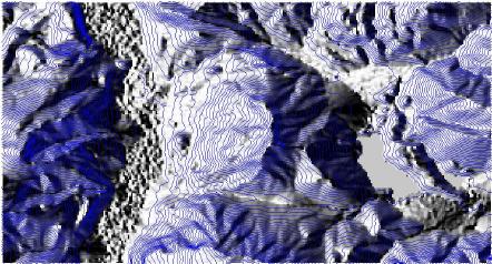
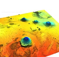
- Olympus Mons (Mars) topography viewed with NVIZ
Example
g.region rast=elevation.10m
nviz elev=elevation.10m
Raster 3D Volumes (voxels)
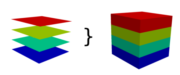
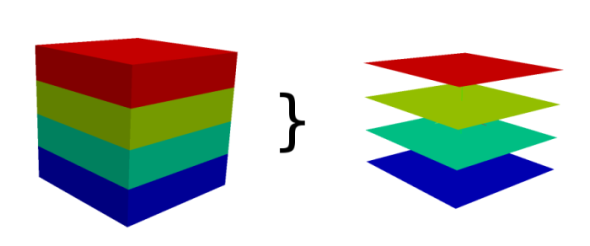
A voxel is jargon for volumetric pixel and means a small 3D cube of size containing one cell of data. See also Voxel. Support for 3D rasters (voxels) is primarily handled by the r3.* modules. A 3D raster can be thought of as a stack of 2D raster maps forming a 3D cube of data cells.
GRASS GIS offers support for 3D raster voxel volumes. Basic features currently cover:
- 3D import/export
- 3D map algebra
- 3D volumes interpolation (IDW algorithm; RST regularized splines with tension algorithm)
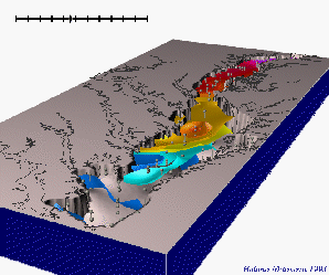
- 3D visualization integrated with NVIZ including voxel volumes and isosurfaces
- 4D visualization using external Vis5D or Paraview software
- Export to VTK: You can visualize this file with the VTK Toolkit, Paraview and MayaVi which are based on VTK.
See also:
The third dimension need not be limited to "z" elevation! It can just as well represent the time dimension in a time series of 2.5D raster surfaces. It is possible to make a 4D visualization using the NVIZ software's animation panels and movie making facility.
You can construct a 3D raster from a series of 2D slices (r.to.rast3), interpolated from 3D vector points (v.vol.rst), or from a text file (r3.in.ascii and r3.in.xyz). You can import from V5D format with r3.in.v5d and export to VTK format with r3.out.vtk (for visualization software like Paraview or VisIt).
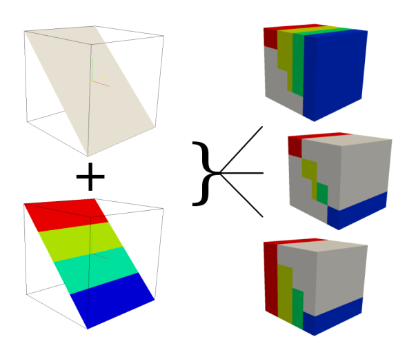
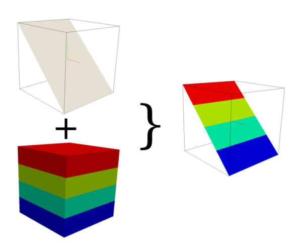
NVIZ supports visualizing 3D raster maps with cutting planes and isosurfaces.
Screenshots
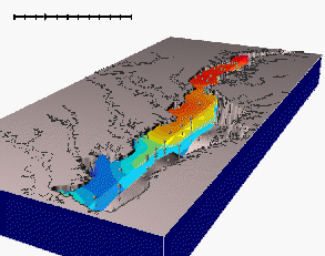
- Chesapeake Bay Nitrogen Levels (4D) from NCSU GMS Lab (Mitasova et al.)
Region settings
Region settings are handled by the g.region module. Special 3D raster controls for g.region include:
-3 flag:  Prints 3D settings
 rast3d   Set region to match this 3D raster map (both 2D and 3D values)
      t   Value for the top edge
      b   Value for the bottom edge
   res3   3D grid resolution (north-south, east-west and top-bottom)
  tbres   Top-bottom grid resolution 3D
Tips
- From the mailing list: Raster 3D from DEMs (drillhole data)
Examples
- Custom volume creation. Here is a small Octave (Matlab) script to create a text file suitable for loading as a 3D raster with r3.in.ascii. Here is the file that this script creates: vox_data50.txt.gz
% f(x,y,z) = x + (y^2 /2) + z^2
x= y= z= 50;

cd ~/grass/
fp = fopen('vox_data50.txt', 'wt')

fprintf(fp, 'north: %d\n', y);
fprintf(fp, 'south: 0\n');
fprintf(fp, 'east: %d\n', x);
fprintf(fp, 'west: 0\n');
fprintf(fp, 'top: %d\n', z);
fprintf(fp, 'bottom: 0\n');
fprintf(fp, 'rows: %d\n', y);
fprintf(fp, 'cols: %d\n', x);
fprintf(fp, 'levels: %d\n', z);

for dep = 1:z
  for row = 1:y
    for col = 1:x
       fprintf(fp, '%.4f', col + (row^2 /2) + dep^2 );
       if(col < 50)
          fprintf(fp, ' ');
       end
    end
    fprintf(fp, '\n');
  end
  disp(['dep ' num2str(dep)])
  fflush(stdout);
end
fclose(fp)
Load the data with:
r3.in.ascii in=vox_data50.txt out=vox50
display isosurfaces with:
g.region rast3d=vox50
nviz -q
Panel->Raster volumes
[New] vox50
Isosurface [Add] [New Constant] 500 [Accept]
 (repeat for 1000,2000,3000)
Change main view height to 125.00 (manual entry)
extract a slice to a 2D raster map with:
g.region t=26.0 b=25.0
r3.to.rast in=vox50 out=vox50x
Vector 3D point data
Historical note: known as "site data" in GRASS GIS 5
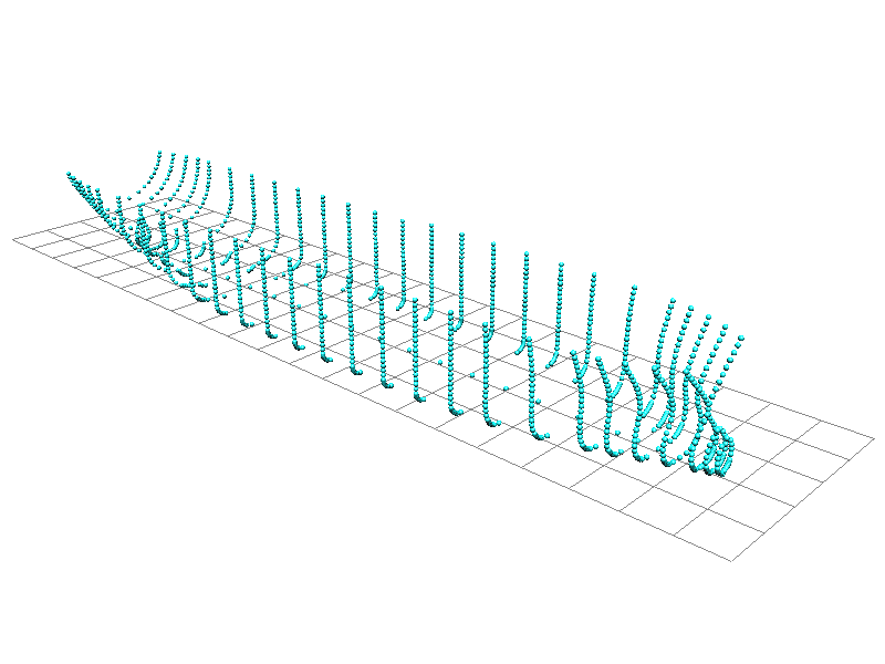
In the "typical" case, "z" data is stored as a non-spatial attribute in a vector point map. In GRASS 6 it is possible to create 3D vector files, i.e. points exist in 3D space.
Import
- Import x,y,z,... data as 3D with the v.in.ascii "-z" flag and "z=" column parameter:
v.in.ascii -z format=point cat=1 x=2 y=3 z=4
- You can convert a 2D vector into a 3D vector with v.extrude (take elevation values from vector attribute column) or v.drape (interpolate elevation values from a raster DEM map).
- It may be more convenient to import massive datasets (millions and millions of points) with r.in.xyz to create a 2.5D raster map.
Conversion to 3D raster volume
- Use the v.vol.rst module to interpolate 3D vector points into a 3D raster volume.
Screenshot
3D points defining the hull of a ship, visualized using NVIZ
Example
TODO: import star guide and display using NVIZ, using magnitude column in database table for dynamic sizing. Requires a "Free" dataset, if you have any leads, please add links to this wiki page. Thanks.
Vector 3D lines
The GRASS vector engine is fully 3D aware, so 3D lines such as highways which cross at a bridge, but do not touch, can be modelled.
- The v.in.dxf or v.in.dwg modules can import 3D vector surfaces. DXF files are usually imported without georeference. To move into the geo-space of the rest of your data they must be projected with v.proj or translated with v.transform.
- 3D line objects can be displayed with NVIZ
- (place above a 2D raster isosurface)
Vector 3D polygons
In the "typical" case, "z" data is stored as a non-spatial attribute in a vector point map. In GRASS 6 it is possible to create 3D vector files, i.e. lines and polygons exist in 3D space. The topological nature of GRASS 6's vector engine means that roads can cross via a bridge without topologically meeting.
- 3D feature types
- face: The 3D equivalent of a boundary. These combine to form a volume surface (e.g. a teapot)
- kernel: The 3D equivalent of a centroid (infrastructure for kernels is in place, but they are currently mostly unused)
- volume: An enclosed 3D space. The 3D equivalent to GRASS's area vector feature, meaning an alias to a "face(s)+kernel" set. (some infrastructure and place-holders exist, but not much in the way of practical applications has been coded yet)
- The v.in.ascii -z flag must be used to create a 3D file
- The v.in.dxf or v.in.dwg modules can import 3D vector surfaces. DXF files are usually imported without georeference. To move into the geo-space of the rest of your data they must be projected with v.proj or translated with v.transform.
If working with them alone, it is recommended to use a simple XY location.
- Visualization with NVIZ: vector data must be placed on a raster surface or constant surface. It may be useful to set the transparency attribute of the raster surface to something unobtrusive.
Getting data and data conversion
There are many free 3D mesh files available for research purposes from INRIA.fr's GAMMA project. These can be converted from e.g. 3D Studio (.3ds) format into DXF files with a converter program like [1] (runs well in Linux under wine). Then use v.in.dxf. Also Blender does a nice job for exporting to 3D DXF.
wcvt2pov.exe supported file formats
- load: AOFF (*.geo), AutoCAD DXF (*.dxf), 3D Studio (*.3ds), Neutral File Format (*.nff), RAW (*.raw), TPOLY (*.tpo), True Type Font (*.ttf), Wavefront (*.obj), World Toolkit (*.nff)
- save: AutoCAD DXF (*.dxf), 3D Studio (*.asc), Neutral File Format (*.nff), Povray V2.2 (*.pov), Povray V2.2 Include (*.inc), RAW (*.raw), TPOLY (*.tpo), True Space (*.cob), VRML V1.0 (*.wrl), Wavefront (*.obj), World Toolkit (*.nff)
Suitable alternative is Open Asset Import Library (short name: Assimp), which is a portable Open Source library to import various well-known 3D model formats in a uniform manner.
Assimp library supported file formats
- import:
Common interchange formats: Collada ( .dae ), Blender 3D ( .blend ), 3ds Max 3DS ( .3ds ), 3ds Max ASE ( .ase ), Wavefront Object ( .obj ), Industry Foundation Classes (IFC/Step) ( .ifc ), XGL ( .xgl,.zgl ), Stanford Polygon Library ( .ply ), *AutoCAD DXF ( .dxf ), LightWave ( .lwo ), LightWave Scene ( .lws ), Modo ( .lxo ), Stereolithography ( .stl ), DirectX X ( .x ), AC3D ( .ac ), Milkshape 3D ( .ms3d ), * TrueSpace ( .cob,.scn )
Motion Capture Formats: Biovision BVH ( .bvh ),* CharacterStudio Motion ( .csm )
Graphics Engine Formats: Ogre XML ( .xml ), Irrlicht Mesh ( .irrmesh ), * Irrlicht Scene ( .irr )
Other file formats: BlitzBasic 3D ( .b3d ), Quick3D ( .q3d,.q3s ), Neutral File Format ( .nff ), Sense8 WorldToolKit ( .nff ), Object File Format ( .off ), PovRAY Raw ( .raw ), Terragen Terrain ( .ter ), 3D GameStudio (3DGS) ( .mdl ), 3D GameStudio (3DGS) Terrain ( .hmp ), Izware Nendo ( .ndo )
- export:
Collada ( .dae ), Wavefront Object ( .obj ), Stereolithography ( .stl ), Stanford Polygon Library ( .ply )
Extrude 2D polygons to 3D
Screenshots
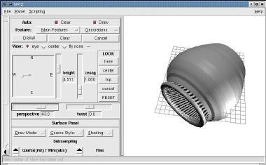
- 3D DXF Mesh object, created in Blender and imported into GRASS (screenshot: A. Bezzi, M. Neteler)
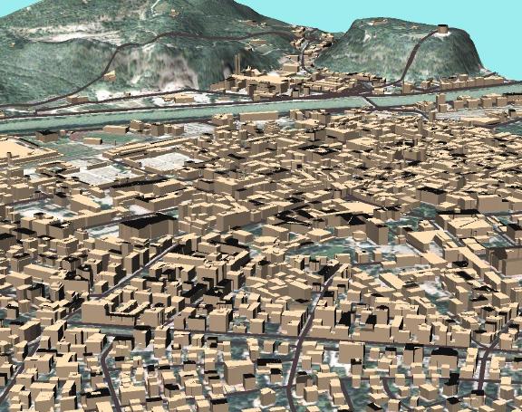
- GRASS: building footprints extruded to 3D blocks (screenshot: M. Neteler)
- (data courtesy City of Trento, Italy - see "Mostra Strumenti Dati" for geodata download)
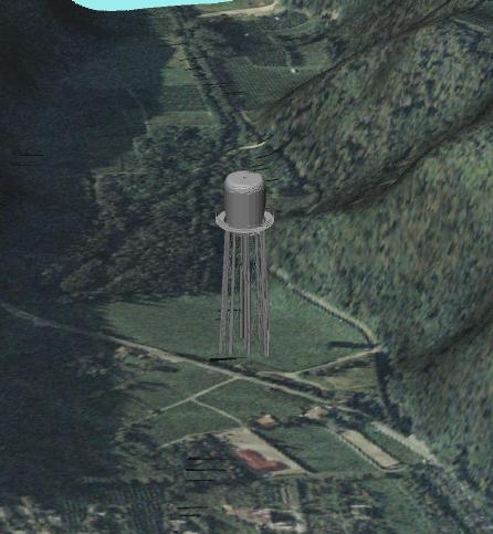
- Watertower imported with v.in.dwg (or use v.in.dxf) displayed over a 2.5D raster surface with color orthophoto raster providing ground coloration.
Pyramid example
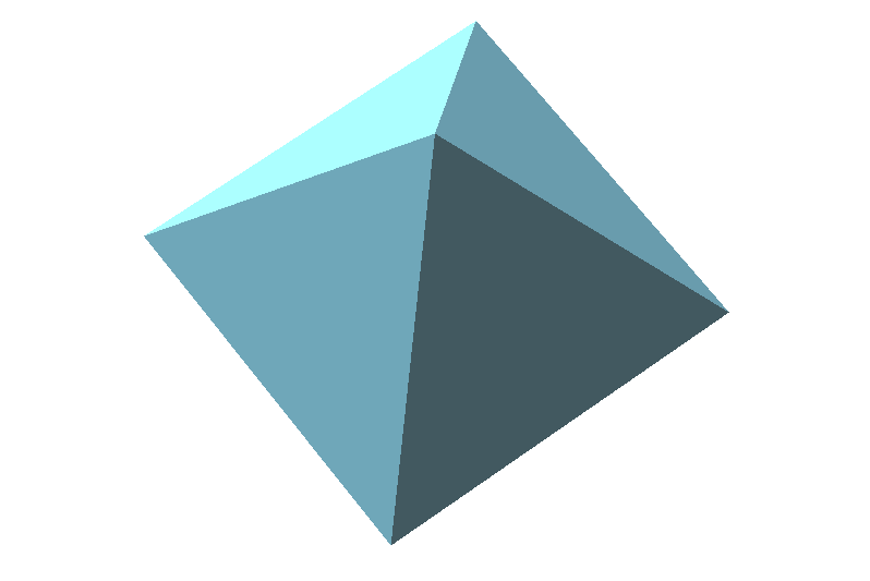
The following is an example of 3D vector surfaces in GRASS ASCII vector format. Can be loaded with v.in.ascii.
# 3D Pyramid in GRASS:  (kernel type still mostly unused in GRASS 6)
#
#  v.in.ascii in=pyramid.vasc out=pyramid_3d format=standard -nz
#  g.region n=150 s=-50 w=-50 e=150 res=10
#  r.mapcalc "one = 1"
#
# GRASS 6
#  nviz elev=one vect=pyramid_3d
#
# or in GRASS 7
#   (m.nviz.image available in both, Command line nviz only in G6)
#
# m.nviz.image -a elevation_map=one@3Dmapset mode=fine resolution_fine=6 \
#   color_map=one@3Dmapset position=0.26,0.82 height=800 perspective=9 \
#   twist=0 zexag=1.0 focus=95,95,1 light_position=-0.03,0.63,0.58 \
#   light_brightness=98 light_ambient=83 light_color=255:255:255 \
#   output=pyramid_3d format=ppm size=798,533 \
#   vline=pyramid_3d vline_color=109:189:215
#
#  tip: in nviz try setting the raster surface transparency to 50%
#
#
F 5
 0 0 10
 0 100 10
 100 100 10
 100 0 10
 0 0 10
F 4
 0 0 10
 50 50 80
 100 0 10
 0 0 10
F 4
 0 100 10
 50 50 80
 0 0 10
 0 100 10
F 4
 100 100 10
 50 50 80
 0 100 10
 100 100 10
F 4
 100 0 10
 50 50 80
 100 100 10
 100 0 10
K 1 1
 40 50 40
 1 1
Stereograms and Anaglyphs
- See the Stereo anaglyphs and Stereoscopic analysis wiki pages, and the d.anaglyph addon module.
Visualization Tools and export
- NVIZ: GRASS's own n-dimensional visualization suite
- wxNviz: wxGUI 3D view mode extension
- voxel output to VTK & Paraview (r.out.vtk, r3.out.vtk, v.out.vtk)
- GRASS and Paraview
- Screenshots (seek Para* there)
- output to Vis5D (r3.out.v5d)
- output to VRML (3D virtual reality) (r.out.vrml)
- output to DXF (Blender, AutoCAD, ...) (v.out.dxf)
Raster 3D (voxel) sample data set
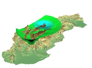
You can download the Slovakia 3D precipitation data from the sample data page ("Slovakia 3D precipitation data set"). For instructions, read the related README file.
Vis5D data viewer
See: GRASS and Paraview software
Vis5D data viewer
(This is an outdated software, Paraview is recommended)
You can also use Vis5D or Vis5d+ to visualize your 3D data set (use r3.out.v5d to export into Vis5D format). VIS5D is a system for interactive visualization of large 5-D gridded data sets such as those produced by numerical weather models. One can make isosurfaces, contour line slices, colored slices, volume renderings, etc of data in a 3-D grid, then rotate and animate the images in real time. There's also a feature for wind trajectory tracing, a way to make text anotations for publications, support for interactive data analysis, etc.
See also
- [2] Multidimensional interpolation and visualization (Mitasova et al., experimental version from USA CERL 1993-95)
- [3] Interpolation and visualization from 3D and 4D scattered data using GRASS GIS (Mitasova et al., experimental version from USA CERL 1993-95)
- Grid3D library was developed by CERL and GMSL/University of Illinois
