Contour lines to DEM: Difference between revisions
m (→About) |
|||
| Line 5: | Line 5: | ||
This page will demonstrate and compare a number of different methods of converting vector contour lines into raster DEM surfaces. | This page will demonstrate and compare a number of different methods of converting vector contour lines into raster DEM surfaces. | ||
Click on images to make them bigger. You may want to download them all at full resolution and then play them back in a quick slide show to highlight the differences. (Images were created | Click on images to make them bigger. You may want to download them all at full resolution and then play them back in a quick slide show to highlight the differences. (Images were created in [[NVIZ]] at 7x vertical exaggeration) | ||
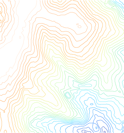
We will use the [[Sample_datasets|North Carolina sample dataset]]'s <tt>elev_lid792_cont1m</tt> 1m contour line map as the starting point. | We will use the [[Sample_datasets|North Carolina sample dataset]]'s <tt>elev_lid792_cont1m</tt> 1m contour line map as the starting point. | ||
Revision as of 16:15, 27 February 2010
About
This page will demonstrate and compare a number of different methods of converting vector contour lines into raster DEM surfaces.
Click on images to make them bigger. You may want to download them all at full resolution and then play them back in a quick slide show to highlight the differences. (Images were created in NVIZ at 7x vertical exaggeration)
We will use the North Carolina sample dataset's elev_lid792_cont1m 1m contour line map as the starting point.
First we set the computational region to match the contour lines vector map, and then we force the resolution to align with a 1m grid:
g.region vect=elev_lid792_cont1m
g.region res=1 -ap
We can display it on a Xmonitor to be sure:
d.mon x0
d.vect elev_lid792_cont1m -z zcolor=haxby
A number of the r.surf.* modules want the input data to be in raster form already, so we rasterize the contour lines, using the level column for the height values. Also some of the older r.surf.* modules only like to work on integers, so to preserve sub-meter fidelity we do a little trick where we multiply by a large number, do the process, then divide by that number again.
v.to.rast in=elev_lid792_cont1m out=elev.1mcont \
  type=line column=level
r.mapcalc "elev.1mcont.100k = elev.1mcont * 100000"
r.surf.idw
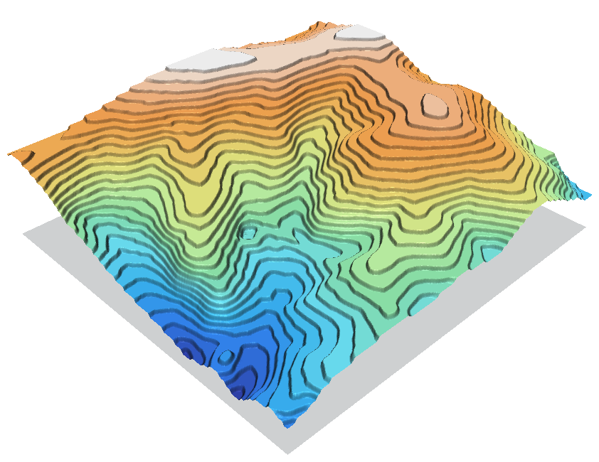
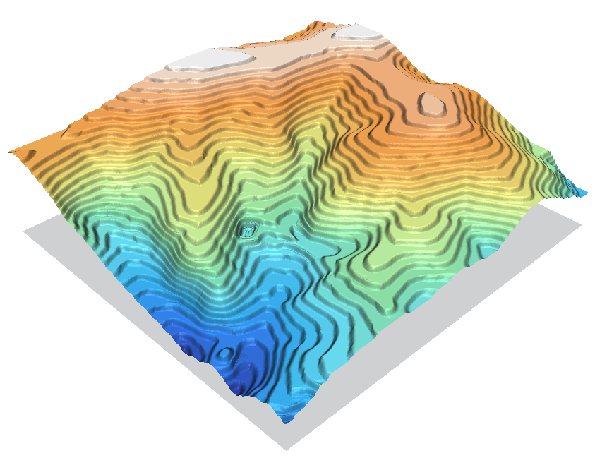
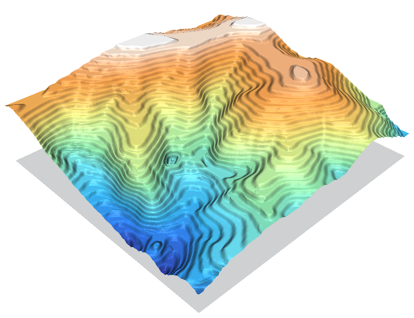
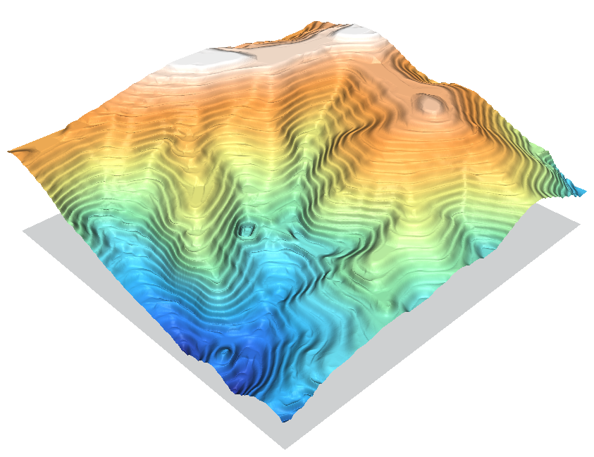
r.surf.idw (and r.surf.idw2) perform inverse distance weighting interpolation, using the n-closest data points to calculate the elevation of a cell, with the closest points having the greatest weight. As we have already converted to raster in the above v.to.rast step, the data points are evenly spaced in our 1m grid. As we expand the number of search points so that it reaches the next contour line, the lines begin to blur together.
r.surf.idw is much faster but does not create floating-point maps directly. Otherwise the module output is practically identical.
  |
  |
 |
As you can see, r.surf.idw creates a rather terraced DEM so won't be too useful for contour line → DEM tasks. On the other hand, if you look at the central valley it does preserve the overland path of the stream quite well.
Commands used:
NPOINTS=36
r.surf.idw in=elev.1mcont.100k out=elev.1mcont.idw.100k npoints=$NPOINTS
r.mapcalc "elev.1mcont.idw_$NPOINTS = elev.1mcont.idw.100k / 100000.0"
g.remove elev.1mcont.idw.100k
r.colors elev.1mcont.idw_$NPOINTS color=haxby
r.surf.nnbathy
The next method we will look at is the r.surf.nnbathy add-on module. It performs a Natural Neighbor interpolation. (see also v.voronoi and v.delaunay)

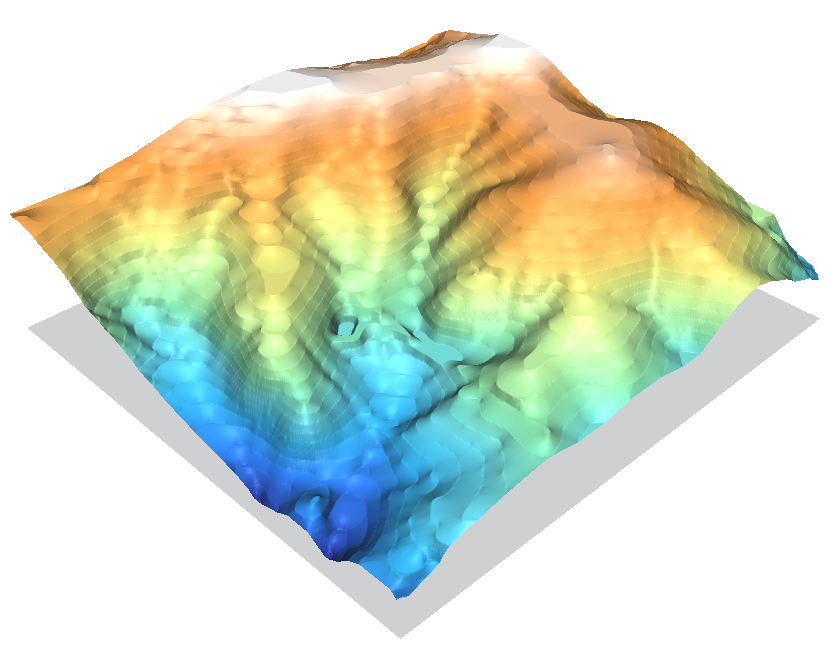
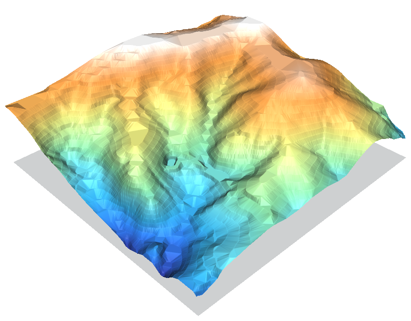
The two NN interpolations do a reasonable job, with a very nice curved surface in the interpolated areas but contour line artifacts are still clearly visible. If you look closely at the peaks and basins you will notice the minor tension/curvature difference between the two. You can get an idea from this of the very nice DEMs you can create given a good spread of input points to work with instead of contour lines.
The linear TIN operation is very fast, but otherwise creates a low quality DEM compared to the other methods which are able to fill the voids between know data points with curves instead of a flat surface.
If you examine the main valley up the center of the image you will notice all 3 methods have nasty step artifacts along the path of the stream.
Unfortunately nnbathy relies on the Triangle library, which is only licensed for non-commercial use. Otherwise it would be added as a core module in the main GRASS distribution.
