V.generalize tutorial/id
This page is in progress of translating to Bahasa Indonesia from English.
MODUL
v.generalize
TUTORIAL
Pendahuluan
Tutorial ini menggambarkan dan menjelaskan tentang kegunaan modul vektor GRASS v.generalize. Modul ini mengimplementasikan operasi generalisasi untuk peta vektor GRASS. Topis yang dibahas dalam tutorial ini adalah : simplifikasi, smoothing, generalisasi jaringan dan perubahan posisi. Untuk penjelasan dasar mengenai operasi ini silakan lihat halaman v.generalize atau yang lebih lengkap lagi lihat McMaster dan Shea (TODO: tambahkan literatur).
Disarankan untuk membaca halaman resmi manual sebelum membaca dokumen ini, atau baca kedua dokumen sekarang juga, karena tutorial ini tidak menjelaskan lebih detil tentang semua parameter input yang ada di manual. Begitu juga sebaliknya, halaman manual tidak disertai dengan contoh yang banyak dan juga tanpa gambar. Dokumen ini juga lebih bersifat sebagai laporan singkat, hasil yang diperoleh dari Google Summer of Code 2007.
Hampir semua contoh dalam dokumen ini menggunakan dataset Spearfish, yang dapat diunduh di sini. Juga, tutorial ini mengasumsikan bahwa pengguna telah menjalankan sesi GRASS dengan location Spearfish dan sebuah window display yang dibuka. Jika Anda mengklik salah satu gambar di sini, ia akan ditampilkan dalam resolusi sebenarnya.
Semua algoritma yang ditampilkan dalam dokumen ini (berusaha tetap) memelihara topologi dari peta input. Artinya, sebagai contoh, metoda smoothing dan simplifikasi tidak pernah menghilangkan titik awal dan terakhir dari garis, dan pemindahan garis tetap mempertahankan persimpangan (junctions) yang dimiliki.
Simplifikasi
v.generalize mengimplementasikan banyak algoritma simplifikasi. Metoda yang paling banyak digunakan adalah algoritma Douglas-Peucker (TODO: literatur). Kita dapat menerapkan algoritma ini untuk sebarang peta vektor dengan cara berikut :
v.generalize input=roads output=roads_douglas method=douglas threshold=50
Penjelasan dari baris perintah di atas adalah : Jalankan v.generalize, terapkan algoritma Douglas-Peucker dengan threshold sama dengan 50 pada peta jalan dan simpan outputnya sebagai peta vektor output_douglas. Baris terakhir dari output garis oleh modul ini :
Number of vertices was reduced from 5468 to 2107[38%]
berarti bahwa berkas input (roads) memiliki jumlah vertex total 5468 dan peta baru(roads_douglas) hanya memiliki 2107 vertex, yang artinya hanya 38% dari aslinya. Dalam contoh lain, jika kita jalankan perintah:
d.vect roads
d.vect roads_douglas col=blue
Kita akan melihat bahwa tidak ada perbedaan signifikan antara peta input dan output. "Only the details were removed".
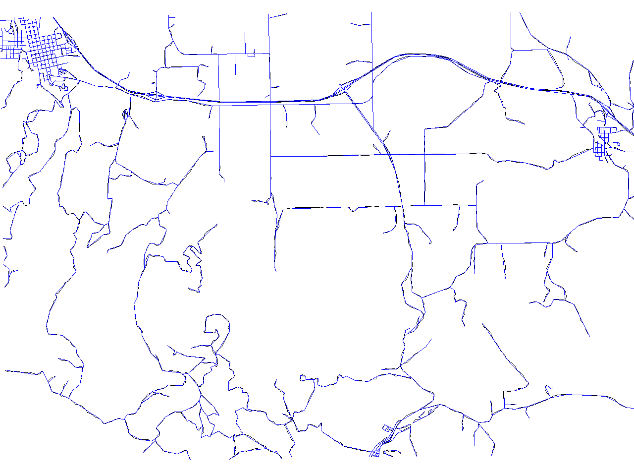
Tingkat kedetilan yang dihilangkan dapat ditentukan dengan parameter : threshold. Ini merupakan contoh bahwa peta output memiliki vertex lebih sedikit dan kedetilan lebih dari threshold tetap dipertahankan. Sebagai contoh, jika kita jalankan
v.generalize input=roads output=roads_douglas method=douglas threshold=200 --overwrite
kita akan mendapatkan sebuah peta dengan hanya 1726 verteks. Kerugian dari perintah di atas adalah perintah tersebut tidak pernah menghapus garis. Jika kita juga ingin menghilangkan garis kecil, kita harus menjalankan perintah di atas dengan tambahan -r, hingga garis yang kurang dari threshold dan area dengan luas dibawah threshold akan dihilangkan:
v.generalize -r input=roads output=roads_douglas method=douglas threshold=200 --overwrite
Pada kasus ini, roads_douglas hanya memiliki 850 verteks dan 387 garis dibandingkan pada peta aslinya (roads) yang memiliki 825 garis. Dalam kasus ini, peta output memiliki detail yang lebih sediki tetapi bentuk dasar dan topologinya tetap dipertahankan:
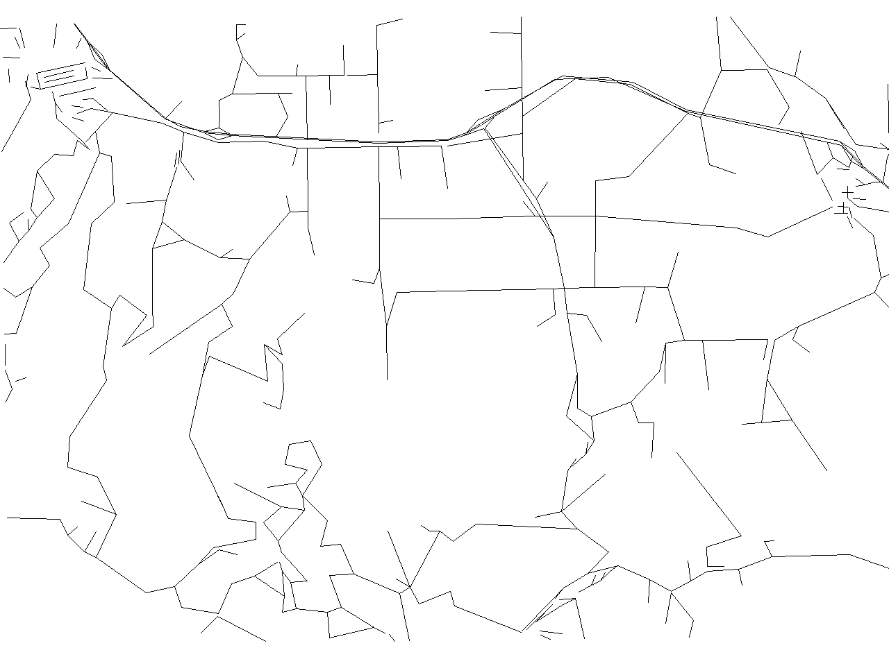
Juga mungkin untuk hanya menghilangkan garis/area kecil saja (tanpa simplifikasi). Hal ini bisa dicapai dengan method=remove_small:
v.generalize input=roads output=roads_remove_small method=remove_small threshold=200
yang menghasilkan peta dengan 399 baris (Perhatikan bahwa garis yang dihilangkan berada di sebelah kiri atas)

Douglas-Peucker Algorithm has very reasonable results, but it is very hard to find(guess) the right value of threshold. Moreover, it is also impossible to simplify each line to (for example) 40%. Exactly for such cases, v.generalize provides method=douglas_reduction. This algorithm is a modification of Douglas-Peucker Algorithm which takes another paratemer reduction which denotes (approximate) simplification of lines. For example,
v.generalize input=roads output=roads_douglas_reduction method=douglas_reduction \
  threshold=0 reduction=50 --overwrite
d.erase
d.vect roads_douglas_reduction
produces following map with 3018 vertices (55%). (Note that there are almost no differencies between the original and the new map)
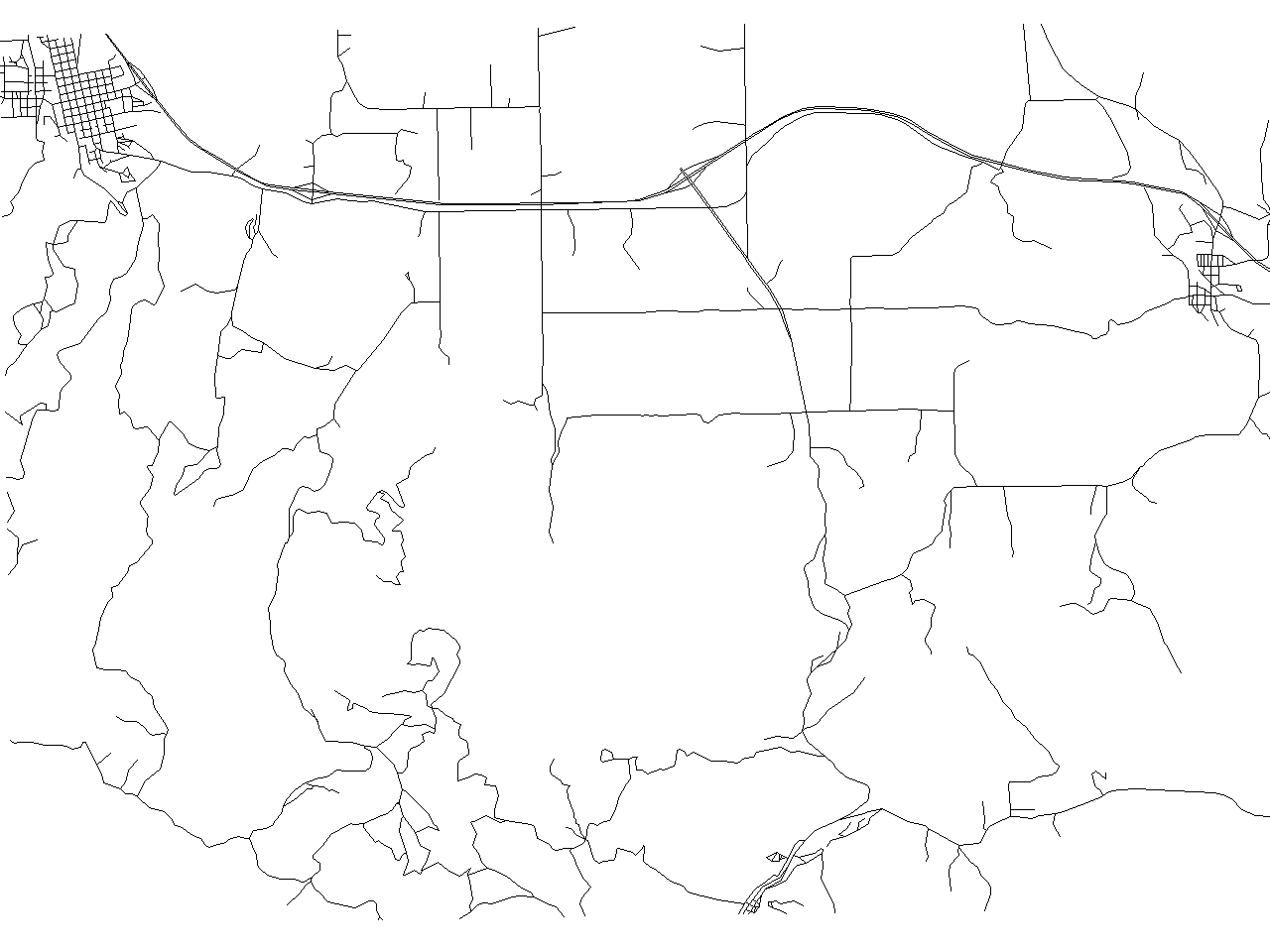
Also observe that the following commands are equivalent
v.generalize input=in output=out method=douglas threshold=eps
v.generalize input=in output=out method=douglas_reduction threshold=eps reduction=100
Another algorithm implemented in this modules is "Vertex Reduction". This algorithm removes the consecutive poins (on the same line) which are closer to each other than threshold. For example,
v.generalize input=in output=out method=reduction threshold=0
removes duplicate points. More precisely, if two consecutive points have the same coordinates then the second point is removed and the first is preserved. The last two algorithm implemented by this module are "Lang" and "Reumann-Witkam" algorithm. For more information about these two algorithms, please see the v.generalize man page. File:Contoh.jpg
Results
The following four pictures show the results obtained by Reumann, Douglas, Lang and Vertex Reduction algorithm resp. The algorithms were run with threshold set to 50 and Lang algorithm with look_ahead=7.
- Simplification algorithms
-
Reumann-Witkam algorithm result containing 2522 [46%] points
-
Douglas algorithm result containing 2107 [38%] points
-
Lang algorithm result containing 2160 [39%] points
-
Vertex Reduction algorithm result containing 4296 [78%] points
The map produced by
- Reumann-Witkam algorithm contains 2522 [46%] points,
- Douglas: 2107 [38%] points,
- Lang: 2160 [39%] and
- Vertex Reduction: 4296 [78%].
Smoothing
v.generalize also supports many smoothing algorithm. For basic descriptions, please consult the v.generalize man page.
Probably, the best results are produced by "Chaiken", "Hermite" and "Snakes" algorithms/methods. However, the remaining algorithms may also produce very reasonable results. Although the Chaiken and Hermite methods may produce the maps with a lot of new points, the methods presented above (simplification) provide a good tool for tackling this problem.
If we run the following command
v.generalize input=roads output=roads_chaiken method=chaiken threshold=1
we get a new map with 33364[640%] vertices.
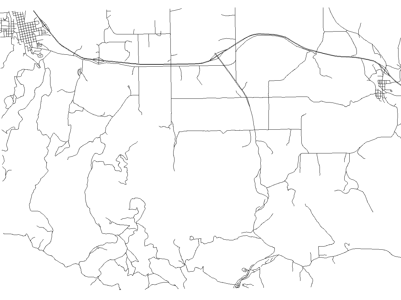
This map looks almost exactly the same as the original map at the current level of detail as the picture below shows. This pictures was produced by the command:
d.erase
d.vect roads
d.vect roads_chaiken col=blue
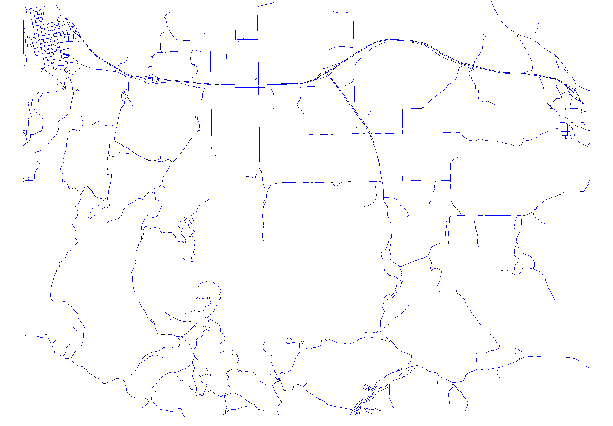
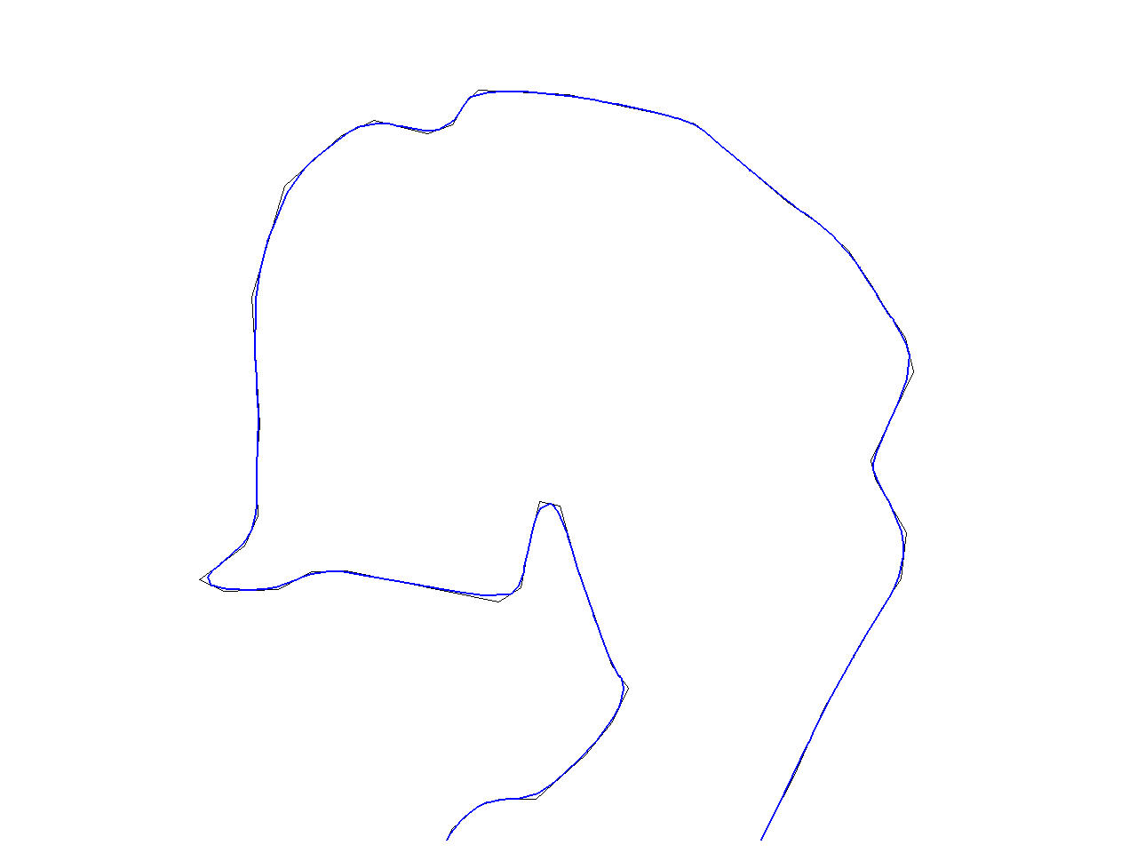
However, if we zoom to a small region, we can see that the new map consists of smooth(er) lines which (very reasonable) approximate the original ones.
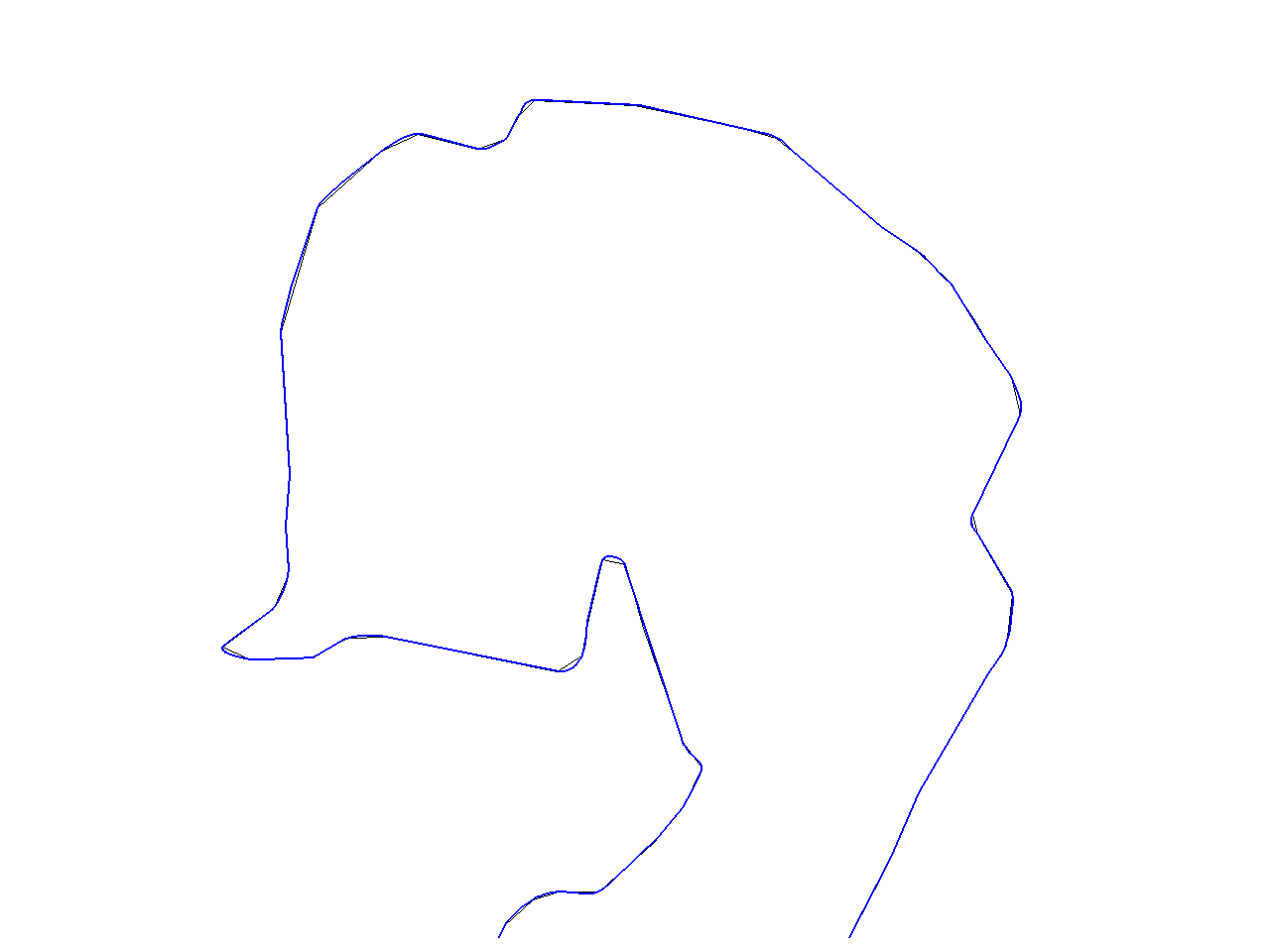
If we apply "Hermite" method instead, we will obtain a map with 14640[267%] vertices.
v.generalize input=roads output=roads_hermite method=hermite threshold=1
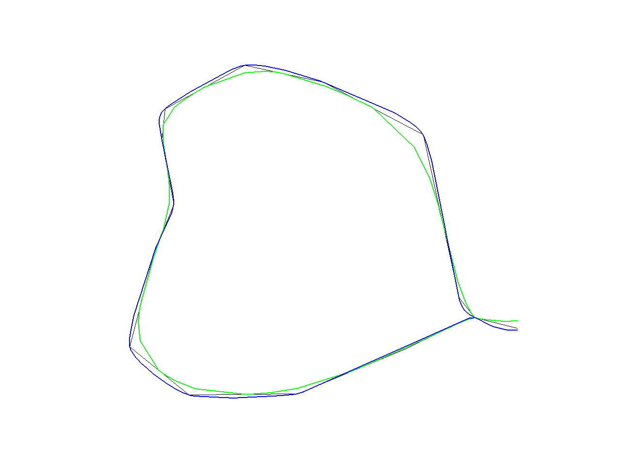
Note, that a difference between "Chaiken" and "Hermite" is that the lines produced by "Chaiken" "inscribe" the orginal lines whereas the "Hermite" lines "circumscribe" the original lines as can be seen in the picture below. (Black line is original line, green line is "Chaiken" and blue is "Hermite")
The algorithms mentioned above are suitable for smooth approximation of given lines. On the other hand, if the aim of smoothing is to "straighten" the lines then the better results are achieved by the other methods. For example,
v.generalize input=roads output=roads_sa method=sliding_averaging look_ahead=7 slide=1
At first sight, we can see that roads_sa contains smooth and straight lines which
preserve the original shape of the lines. This difference is obvious if we zoom to a small
region of a map (see below. Again, original line is black, new line is blue)
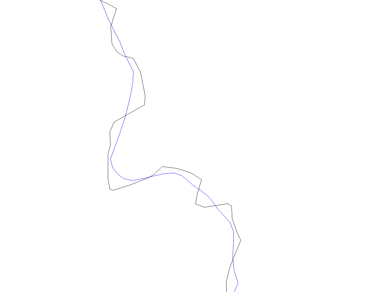
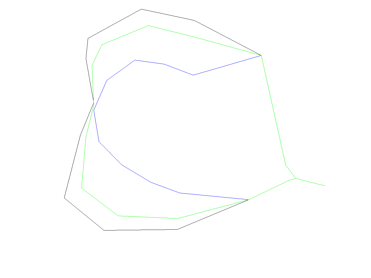
If the lines are "too straight" then we can set "slide" to a smaller value to obtain the lines which better preserve the original shape. In the picture below, original line is black, line produced by "slide=1" is blue and "slide=0.3" is green.
Very similar results can be obtained by Distance Weighting Algorithm (method=distance_weighting). This is not very surprising since these algorithms are almost the same. For example, the image below shows the outputs of "Distance Weighting Algorithm". The image was generated by the following sequence of commands
v.generalize input=roads output=roads_dw1 method=distance_weighting look_ahead=7 slide=1
v.generalize input=roads output=roads_dw2 method=distance_weighting look_ahead=7 slide=0.3
d.erase
d.vect roads
d.vect roads_dw1 col=red
d.vect roads_dw2 col=blue
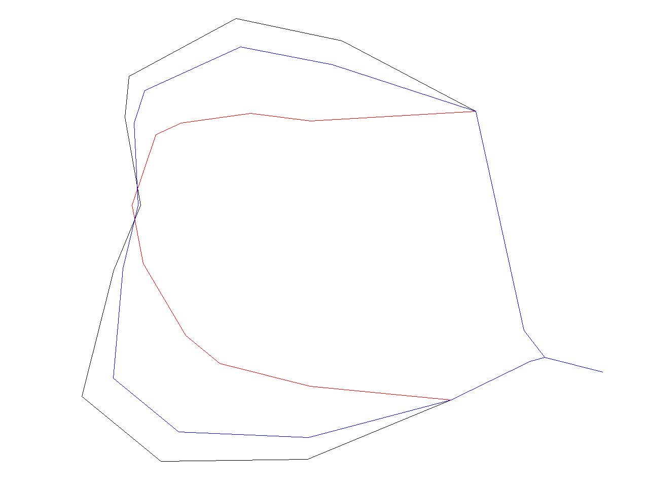
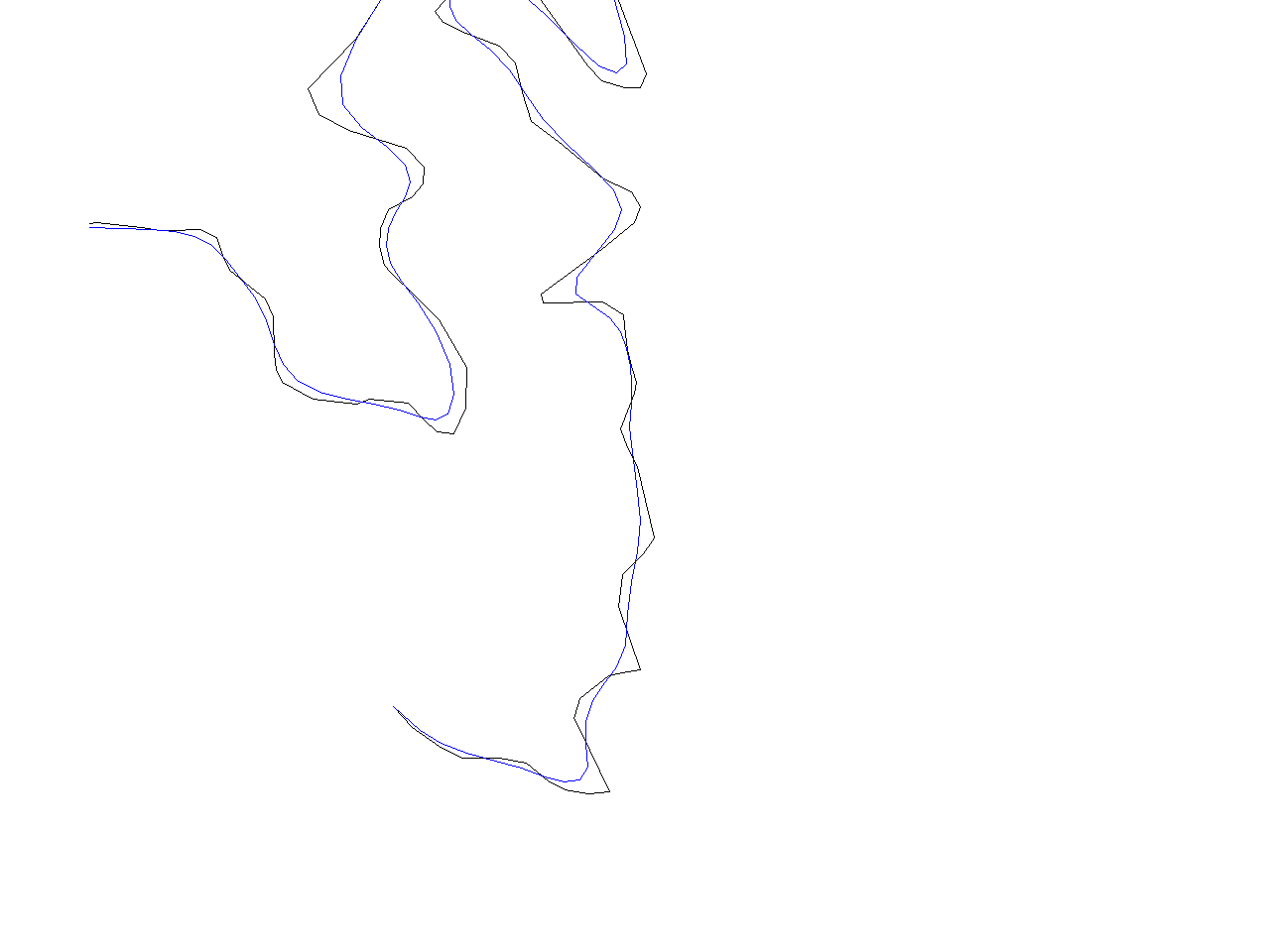
Also, very good resutls can be obtained by the "Snakes" algorithm. On the other hand, it is the (assymtotically) slowest smoothing algorithm implemented in this however. Behaviour of this algorithm is controlled by "alpha" and "beta" parameter. Reasonable range of values for these two parameters is [0..5] where higher values correspond to the straighter lines. Module outputs the input map if alpha=beta=0. And this command
v.generalize input=roads output=roads_snakes method=snakes alpha=1 beta=1
produces a map containing following region (original line is black)
Last smoothing algorithm implemented in this module is "Boyle's Forward-Looking Algorithm" which is another "straightening" algorithm.
v.generalize input=roads output=roads_boyle method=boyle look_ahead=5
produces a map containing following region (original line is black)
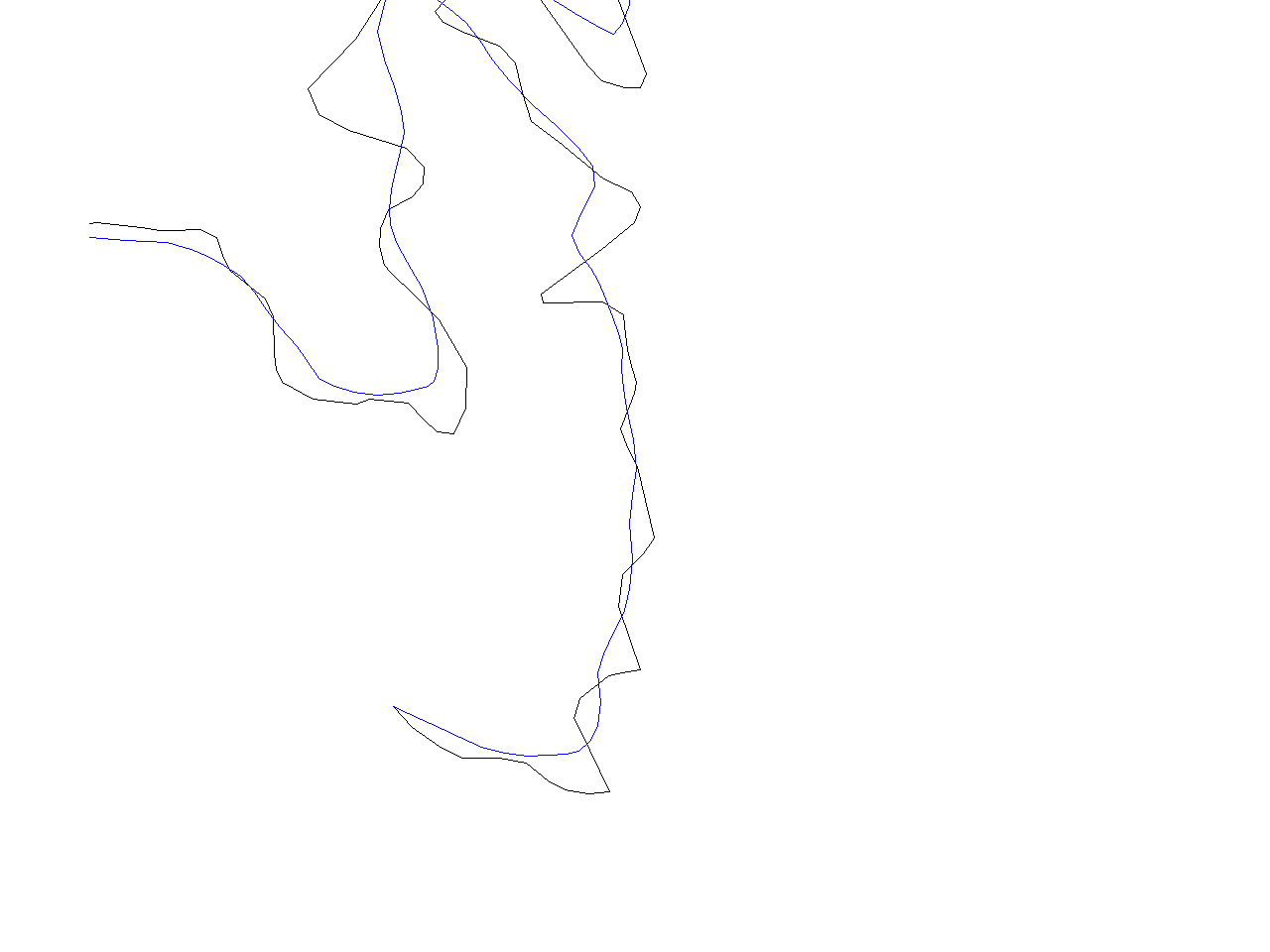
Area smoothing example
# spearfish
g.region rast=geology
r.reclass in=geology out=geology.claysand << EOF
8 = 8 claysand
EOF
r.to.vect in=geology.claysand out=geology_claysand feature=area
v.generalize in=geology_claysand out=geology_claysand_smooth method=snakes
Displacement
If we render entire Spearfish location, we can see in the upper half of the map two interstates which overlap. This is not logically correct (I hope, they do not evarlap in real) and it is also considered as an (presentation) error. For solving such problems, v.generalize provides "dislplacement" method. As the name suggests, this method displaces linear features which are close to each other so that they do not overlap/collide. Method implemented in this modules (based on Snakes) has very good results but not very good perfomance. Therefore the calculations may take few(several) minutes. For this reason, displacement is applied to the simplified lines in this document.
v.generalize input=roads output=roads_dr method=douglas_reduction threshold=0 reduction=50
v.generalize input=roads_dr output=roads_dr_disp method=displacement alpha=0.01 beta=0.01 threshold=100 iterations=35
First command produces simplified lines and then the second command applied displacement operator to the simplified line. Parameters alpha and beta specifies the rigidity of the lines. This means that displacement is bigger for small values of alpha and beta. Also, the displacement is not very significant for higher(>=1.0) values of alpha, beta. Threshold parameter denotes the critical distance. Only the points (and their neighbours) which are closer than threshold apart are displaced by v.generalize. Module tries to move these points such that they are at least threshold apart. However, the displaced points are never threshold (or more) apart for positive values of alpha and beta. Displacement as implemented in v.generalize is an iterative process. Parameter "iterarions" specifies the number of iterations the collisions between the points are resolved. In general, the quality of displacement increases with the number of iterations. However, quality converges quite rapidly and for all maps I tried, the sufficient value of iterations was between 20 and 50. Two command above produce the picture below. Note that it is now possible to distinguish between two "interastate lines" and also observe the free space between interstate and the lines directly below it.

Network Generalization
Network generalization is suitable for selecting "the most important" subnetwork of a network. For example, to select highways, interstates from a road network. Examples in this section work with new GRASS default dataset, which can be downloaded here.
If we render map "streets_wake" we really cannot see the streets, but the only thing we can see is a big black rhombus. We will try to improve this. Firstly, network generalization requites quite a lot of time and memory. Therefore, we begin with simplification of "streets_wake":
v.generalize input=streets_wake output=streets_rs method=remove_small threshold=50
Then we can begin with network generalization. If we execute the folllowing command:
v.generalize input=streets_rs output=streets_rs_network method=network betweeness_thresh=50
we obtain the following map containing "only" 14128. Original map has 49746
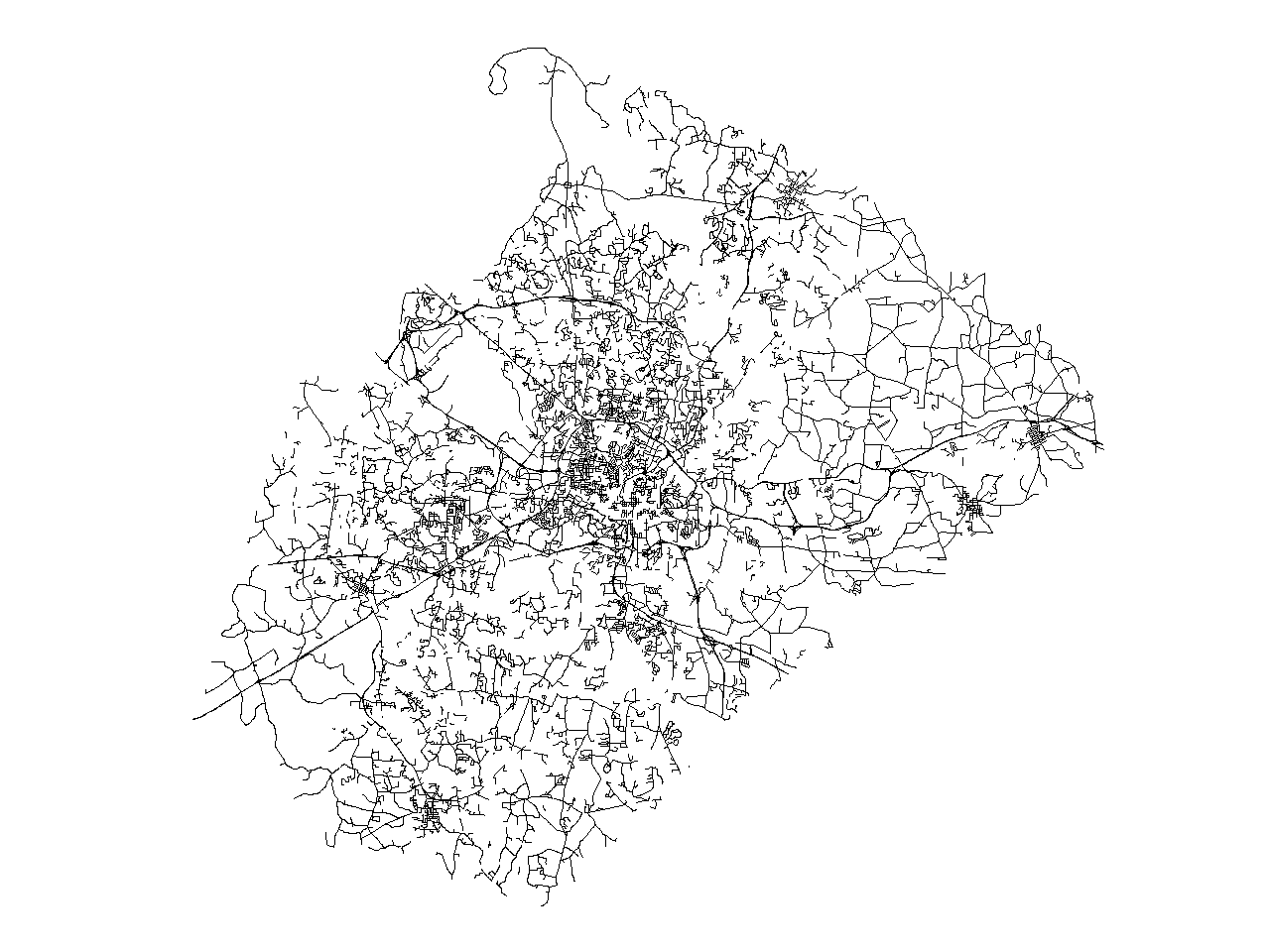
If this is still not enough, we can increase the value of betweeness_thresh to, for example 200. For this value, v.generalize produces following map with 11537 lines.
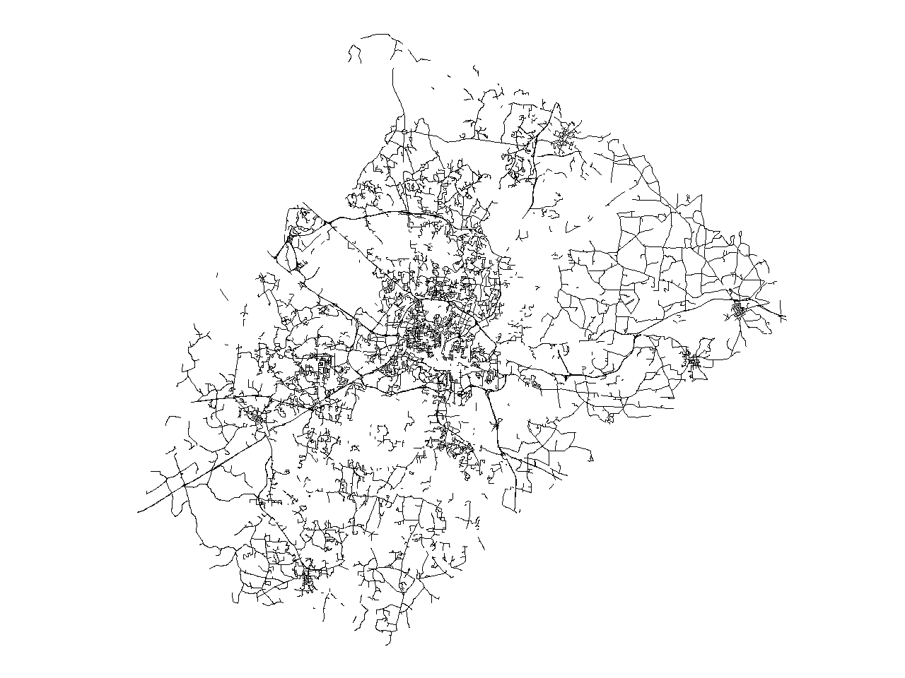
It is also possible to change the values of "closeness_thresh" and "degree_thresh". Parameter "closeness_thresh" is suitable for selecting the "centre(s)" of a network. This parameter is always between 0 and 1. And "reasonable values" of this parameter are smaller for bigger network.
Gereneral Parameters
v.generalize has some parameters and flags which affect the general behaviour of module.
The simplest one is -c flag. "C" stands for copy and if this flag is on then the attributes are copied from the old map to the new map. Note that the attributes of removed features are dropped.
Default behaviour of this module is that the selected algorithm/method is applied to the all lines/areas. It is possible to apply the most of the algorithms only to the selected features. This is achieved by "type", "layer", "cats" and "where" parameters. This works for all algorithms except "Network Generalization" which is always applied to the all features. For example, the following command applies "Douglas Reduction" algorithm to interstates and highways (cat<3) and leaves the other lines unaltered. It also copies the attributes
v.generalize -c input=roads output=roads_douglas_reduction2 method=douglas_reduction threshold=0 reduction=50 type=line where="cat<3"
And the following command removes the small areas
v.generalize input=soils output=soils_remove_small method=remove_small threshold=200 type=area
Similarly, the following command displaces only the interstates (cats=1) and the lines with a different category number are not taken into the account.
v.generalize input=roads output=roads_displacement2 method=displacement \
   threshold=75 alpha=0.01 beta=0.01 iterations=20 cats=1
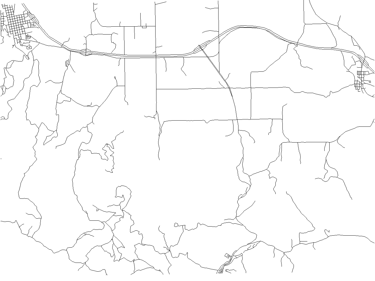
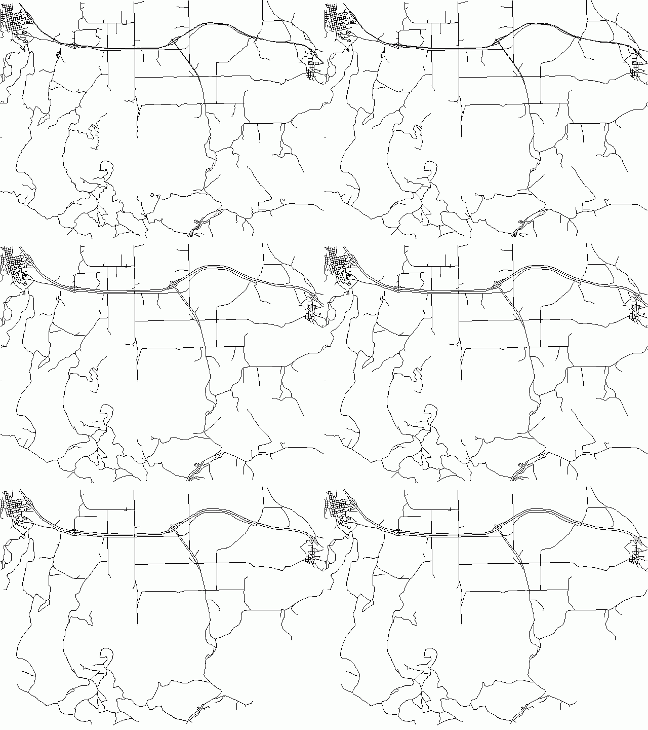
We end up with a complex example of a generalization of "roads" in Spearfish location.
#straighten the lines
v.generalize input=roads output=step1 method=snakes alpha=1 beta=1
#simplification
v.generalize input=step1 output=step2 method=douglas_reduction threshold=0 reduction=55
#displacement
v.generalize input=step2 output=step3 method=displacement alpha=0.01 beta=0.01 threshold=100 iterations=50
#remove small areas
v.generalize input=step3 output=step4 method=remove_small threshold=75
#network generalization
v.generalize input=step4 output=step5 method=network betweeness_thresh=5 closeness_thresh=0.0425
#smoothing
v.generalize input=step5 output=step6 method=chaiken threshold=1
#simplification
v.generalize input=step6 output=step7 method=douglas threshold=1
#remove temporary maps
g.remove vect=step1,step2,step3,step4,step5,step6
The result "step7" has 655 lines and 3545 vertices and the commands above have the following effect:
References
TODO
AUTHORS
- Daniel Bundala, Google Summer of Code 2007, Student
- Wolf Bergenheim, Mentor
![Reumann-Witkam algorithm result containing 2522 [46%] points](/w/images/V.generalize.reumann.png)
![Douglas algorithm result containing 2107 [38%] points](/w/images/V.generalize.douglas.png)
![Lang algorithm result containing 2160 [39%] points](/w/images/V.generalize.lang.png)
![Vertex Reduction algorithm result containing 4296 [78%] points](/w/images/V.generalize.reduction.png)