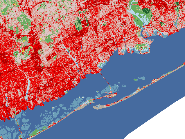
NLCD Land Cover

About
- Raster grid covering the Continental US at 30 meter resolution
From the Spearfish dataset's landcover.30m history file:
- National Land Cover Data Set NLCD, U.S. Geological Survey (USGS)
- The NLCD was compiled from Landsat TM imagery (circa 1992) with a spatial resolution of 30 meters supplemented by various ancillary data (where available). The satellite images were analyzed and interpreted by using very large, sometimes multi-State, image mosaics (that is, up to 18 Landsat scenes). Because a relatively small number of aerial photographs were necessarily conducted from a broad spatial perspective. Furthermore, the accuracy assessments correspond to Federal Regions, which are groupings of contiguous States. Thus, the reliability of the data is greatest at the State or multi-State level. The statistical accuracy of the data is known only for the region.
Obtaining data from the USGS
The classic Spearfish GRASS sample dataset contains a landcover.30m raster map which is an excerpt from an older version of the NLCD dataset.
- Download site: https://www.mrlc.gov/data
- Data is provided in ERDAS Imagine .img format.
- As of April 2019 the zipped dataset is a 1.4 GB.
- Create an Albers location
- this can also be done automatically with the Location Wizard using the downloaded .img file.
Here are the values for the CONUS dataset:
name: Albers Equal Area
proj: aea
datum: wgs84
ellps: wgs84
lat_1: 29.5
lat_2: 45.5
lat_0: 23
lon_0: -96
x_0: 0
y_0: 0
towgs84: 0,0,0,0,0,0,0
no_defs: defined
Importing
Rather than import the entire 16GB raster image, just make a virtual link to it:
r.external in=NLCD_2016_Land_Cover_L48_20190424.img out=NLCD_2016_Land_Cover_L48_20190424 title="Land Cover 2016"
Then use g.region to zoom to your area of interest and r.mapcalc to extract a subset
g.region -p n= s= e= w= res=30 align=NLCD_2016_Land_Cover_L48_20190424
r.mapcalc "NLCD.extract = NLCD_2016_Land_Cover_L48_20190424"
Categories
These can be applied with the r.category module.
0:Unclassified
11:Open Water
12:Perennial Snow/Ice
21:Developed, Open Space
22:Developed, Low Intensity
23:Developed, Medium Intensity
24:Developed, High Intensity
31:Barren Land
41:Deciduous Forest
42:Evergreen Forest
43:Mixed Forest
52:Shrub/Scrub
71:Herbaceous
81:Hay/Pasture
82:Cultivated Crops
90:Woody Wetlands
95:Emergent Herbaceous Wetlands
Colors

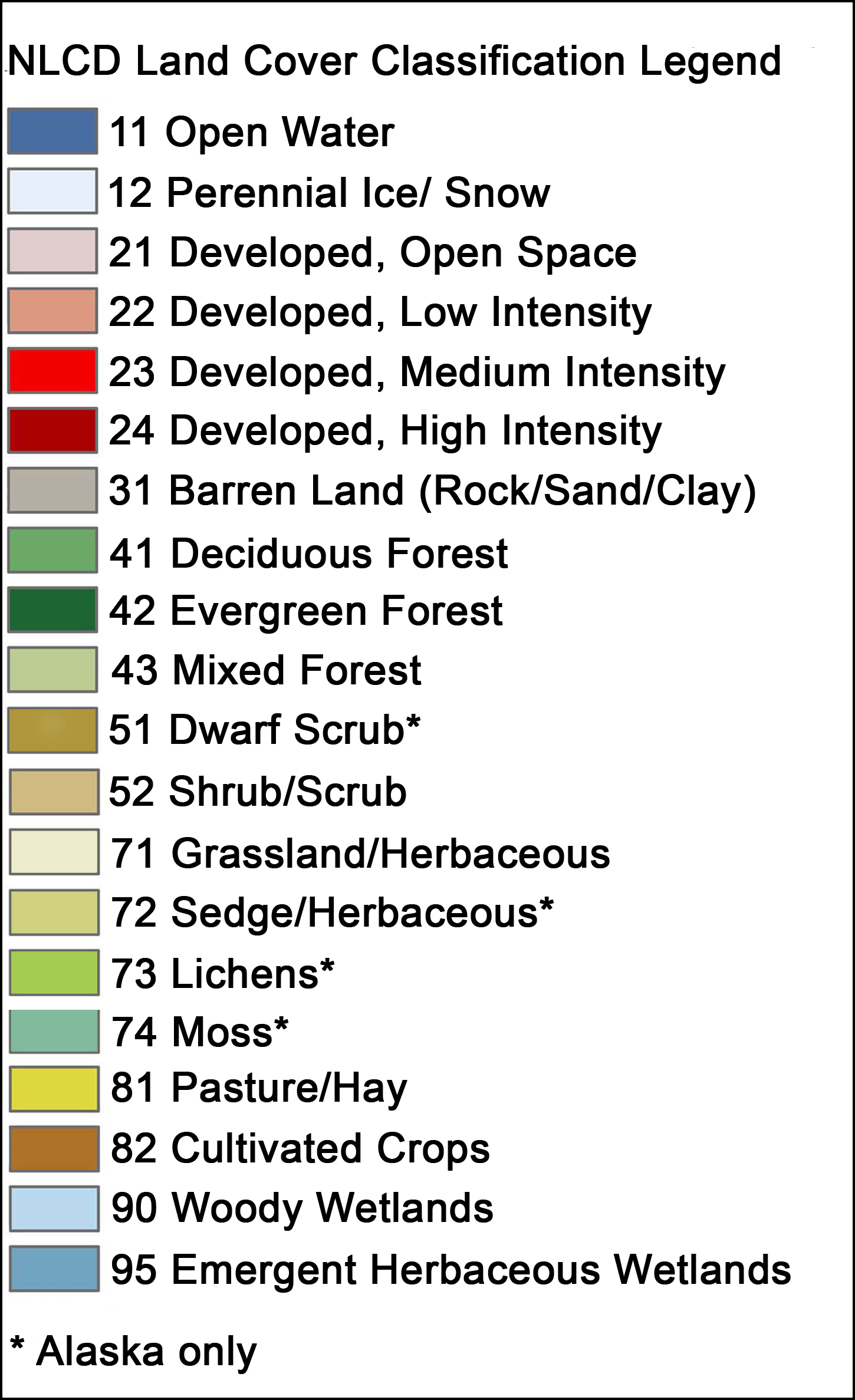
These should load in automatically, but if they don't here are the official colors which you can load in with the r.colors module's rules= option:
11 70:107:159
12 209:222:248
21 222:197:197
22 217:146:130
23 235:0:0
24 171:0:0
31 179:172:159
41 104:171:95
42 28:95:44
43 181:197:143
52 204:184:121
71 223:223:194
81 220:217:57
82 171:108:40
90 184:217:235
95 108:159:184
Legend
Use the -n and -c flags of d.legend to limit the legend to named categories.
Manning's n
For using as a basis for Manning's n friction coefficients, you can make a virtual reclass map with r.reclass. The module will only reclass as integers so the table below is reclassed into parts per ten-thousand. Crop your area of interest with r.mapcalc and divide by 10000.0 at the same time to get the Manning's n number.
Actual values for your location will vary widely, the following is simply a starting point.
0 = 0  Unclassified
11 = 0250 Open Water
12 = 0220 Perennial Snow/Ice
21 = 0400 Developed, Open Space
22 = 1000 Developed, Low Intensity
23 = 0800 Developed, Medium Intensity
24 = 1500 Developed, High Intensity
31 = 0275 Barren Land
41 = 1600 Deciduous Forest
42 = 1800 Evergreen Forest
43 = 1700 Mixed Forest
52 = 1000 Shrub/Scrub
71 = 0350 Herbaceous
81 = 0325 Hay/Pasture
82 = 0375 Cultivated Crops
90 = 1200 Woody Wetlands
95 = 0700 Emergent Herbaceous Wetlands
References:
- Ven Te Chow, 1959 (Corvallis)
- USGS's Guide for Selecting Manning's Roughness Coefficients for Natural Channels and Flood Plains
- Kalyanapu, Alfred & Burian, Steve & Mcpherson, Timothy. (2009). Effect of land use-based surface roughness on hydrologic model output. Journal of Spatial Hydrology. 9. 51-71.
- Liu, Zhu & Merwade, Venkatesh & Jafarzadegan, Keighobad. (2018). Investigating the role of model structure and surface roughness in generating flood inundation extents using 1D and 2D hydraulic models. Journal of Flood Risk Management. e12347. 10.1111/jfr3.12347.
- Bunya, et al.. (2010). A High-Resolution Coupled Riverine Flow, Tide, Wind, Wind Wave, and Storm Surge Model for Southern Louisiana and Mississippi. Part I: Model Development and Validation. Monthly weather review 138.2: 345-377.