Workshop on urban growth modeling with FUTURES
This is material for US-IALE 2016 workshop Spatio-temporal Modeling with Open Source GIS: Application to Urban Growth Simulation using FUTURES held in Asheville April 3, 2016. This workshop introduces GRASS GIS and FUTURES urban growth modeling framework.
Workshop introduction
r.futures.* is an implementation of the FUTure Urban-Regional Environment Simulation (FUTURES)[1] which is a model for multilevel simulations of emerging urban-rural landscape structure. FUTURES produces regional projections of landscape patterns using coupled submodels that integrate nonstationary drivers of land change: per capita demand (DEMAND submodel), site suitability (POTENTIAL submodel), and the spatial structure of conversion events (PGA submodel).
[1] Meentemeyer, R. K., Tang, W., Dorning, M. A., Vogler, J. B., Cunniffe, N. J., & Shoemaker, D. A. (2013). FUTURES: multilevel simulations of emerging urban-rural landscape structure using a stochastic patch-growing algorithm. Annals of the Association of American Geographers, 103(4), 785-807
Software
There are a number of software requirements to run FUTURES that will need to be download and installed. Required software includes:
- GRASS GIS 7
- addons
- R (≥ 3.0.2) - needed for r.futures.potential with packages:
- MuMIn, lme4, optparse, rgrass7
- SciPy - useful for r.futures.demand
Installation
We use the R statistical software for our calculation of site suitability (i.e. development potential) in FUTURES. R is a free software environment for statistical computing and graphics. If you don't have R, or you have older an version, please download and install the software from install R and be sure to additionally add these required packages:
install.packages(c("MuMIn", "lme4", "optparse", "rgrass7"))
Use the instructions bellow to install GRASS GIS. Then, GRASS GIS addons needed for the workshop can be downloaded and installed from a GRASS GIS session:
g.extension r.futures
g.extension r.sample.category
MS Windows
We will be using GRASS GIS 7.0.3 that can be found here in the OSGeo4W package manager. Please install the latest stable GRASS GIS 7 version and the SciPy Python package using the Advanced install option. A guide with step by step screen shot instructions is available here.
In order for GRASS to be able to find R executables, GRASS must be on the PATH variable. Follow this solution to make R accessible from GRASS permanently. A simple but temporary solution is to open GRASS GIS and paste this in the black terminal:
set PATH=%PATH%;C:\Program Files\R\R-3.0.2\bin
This has to be repeated after restarting GRASS session.
Ubuntu Linux
Install GRASS GIS from packages:
sudo add-apt-repository ppa:ubuntugis/ubuntugis-unstable
sudo apt-get update
sudo apt-get install grass
Mac OS X
Install GRASS GIS 7.0.3 using homebrew osgeo4mac:
brew tap osgeo/osgeo4mac
brew install grass-70
Using homebrew install also Python, NumPy, SciPy.
Workshop data
The data that we will be using for the workshop can be download here: sample dataset. Please place these layers in your local GRASS directory:
- digital elevation model (NED)
- NLCD 2001, 2006, 2011
- NLCD 1992/2001 Retrofit Land Cover Change Product
- transportation network (TIGER)
- county boundaries (TIGER)
- protected areas (Secured Lands)
- cities as points (USGS)
In addition, download population information as text files:
- county population past estimates and future projections (NC OSBM) per county (nonspatial)
GRASS GIS introduction
Here we provide an overview of the GRASS GIS project: grass.osgeo.org that might be helpful to review if you are a first time user. For this exercise it's not necessary to have a full understanding of how to use GRASS GIS. However, you will need to know how to place your data in the correct GRASS GIS database directory, as well as some basic GRASS functionality. Here we introduce main concepts necessary for running the tutorial:
Setting up GRASS for the tutorial
GRASS uses unique database terminology and structure (GRASS database) that are important to understand for the set up of this tutorial, as you will need to place the required data (e.g. Location) in a specific GRASS database. In the following we review important terminology and give step by step directions on how to download and place you data in the correct location.
Important GRASS directory terminology
- A GRASS database consists of directory with specific Locations (projects) where data layer are stored
- Location is a directory with data related to one geographic location or a project. All data within one Location has the same coordinate reference system.
- Mapset is a collection of maps within Location, containing data related to a specific task, user or a smaller project
Creating a GRASS database for the tutorial
You need to create a GRASS database with the Mapset that we will use for the tutorial before we can run the FUTURES model. Please download the workshop location, noting where the files are located on your local directory. Now, create (unless you already have it) a directory named grassdata (GRASS database) in your home folder (or Documents), unzip the downloaded data into this directory. You should now have a Location futures_ncspm in grassdata.
-
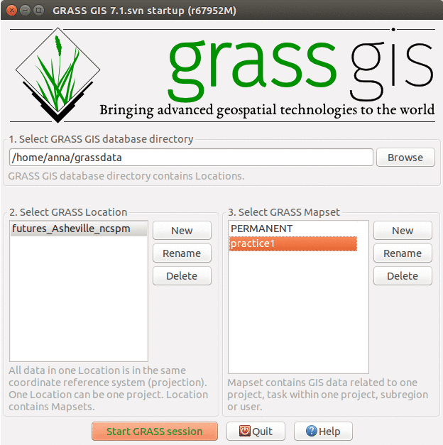
GRASS GIS 7.0.3 startup dialog with downloaded Location and Mapsets for FUTURES workshop

Launching and exploring data in GRASS
Now that we have the data in the correct GRASS database, we can launch the Graphical User Interface (GUI) in Mapset practice1. The GUI interface allows you to display raster, vector data as well as navigate through zooming in and out. Advanced exploration and visualization, like many popular GIS software, is also possible in GRASS (e.g. queries, adding legend). The print screens below depicts how you can add different map layers (left) and display the metadata of your data layers.
-
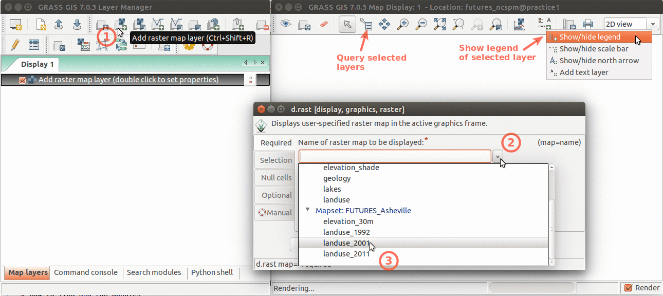
Layer Manager and Map Display overview. Annotations show how to add raster layer, query, add legend.
-
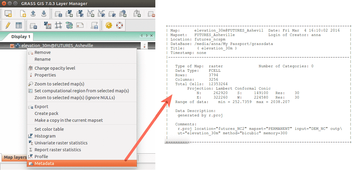
Show raster map metadata by right click on layer


GRASS functionality
One of the advantages of GRASS is the diversity and number of modules that let you analyze all manner of spatial and temporal. GRASS GIS has over 500 different modules in the core distribution and over 230 addon modules that can be used to prepare and analyze data layers.
| Prefix | Function | Example |
|---|---|---|
| r.* | raster processing | r.mapcalc: map algebra |
| v.* | vector processing | v.clean: topological cleaning |
| i.* | imagery processing | i.segment: object recognition |
| db.* | database management | db.select: select values from table |
| r3.* | 3D raster processing | r3.stats: 3D raster statistics |
| t.* | temporal data processing | t.rast.aggregate: temporal aggregation |
| g.* | general data management | g.rename: renames map |
| d.* | display | d.rast: display raster map |
Command line vs. GUI interface
GRASS modules can be executed either through a GUI or command line interface. The GUI offers a user-friendly approach to executing modules where the user can navigate to data layers that they would like to analyze and modify processing options with simple check boxes. The GUI also offers an easily accessible manual on how to execute a model. The command line interface allows users to execute a module using command prompts specific to that module. This is handy when you are running similar analyses with minor modification or are familiar with the module commands for quick efficient processing. In this workshop we provide module prompts that can be copy and pasted into the command line for our workflow, but you can use both GUI and command line depending on personal preference. Look how GUI and command line interface represent the same tool.
Task: compute aspect (orientation) from provided digital elevation model using module r.slope.aspect using both module dialog and command line.
- How to find modules? Modules are organized by their functionality in wxGUI menu, or we can search for them in Search modules tab. If we already know which module to use, we can just type it in the wxGUI command console.
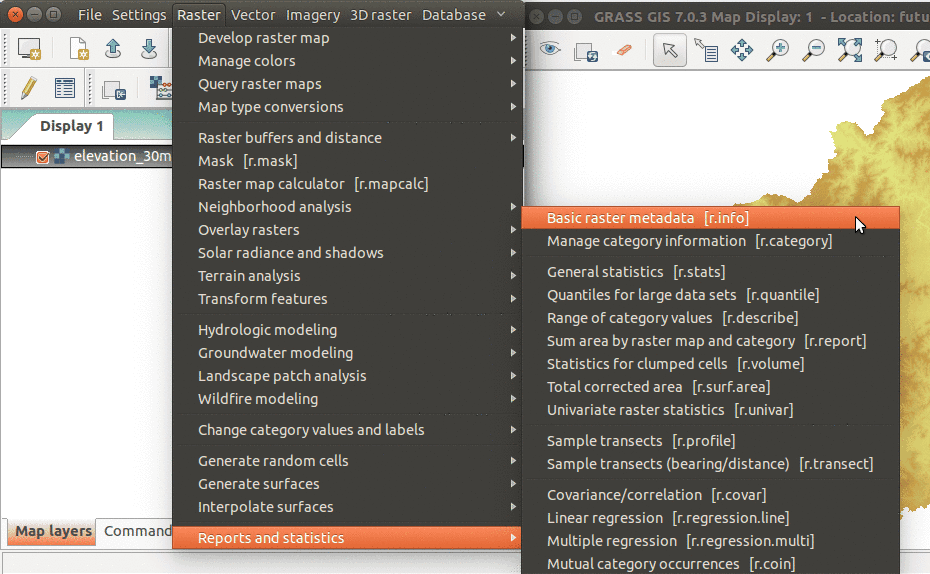
Modules can be found in wxGUI menu
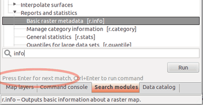
You can search modules by name, description or keywords in Search modules tab
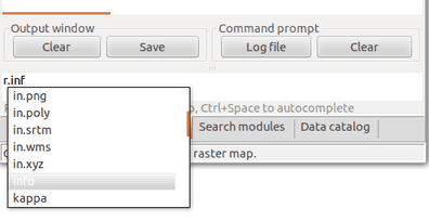
By typing prefix r. we make a list of modules starting with that prefix to show up.


Computational region
Computational region - is an important raster concept in GRASS GIS. In GRASS a computational region can be set, subsetting larger extent data for quicker testing of analysis or analysis of specific regions based on administrative units. We provide a few points to keep in mind when using the computational region function:
- defined by region extent and raster resolution
- applies to all raster operations
- persists between GRASS sessions, can be different for different mapsets
- advantages: keeps your results consistent, avoid clipping, for computationally demanding tasks set region to smaller extent, check your result is good and then set the computational region to the entire study area and rerun analysis
- run
g.region -por in menu Settings - Region - Display region to see current region settings

GRASS 3D view
We can explore our study area in 3D view.
- Add elevation_30m and uncheck or remove any other layers.
- Zoom to an area around Asheville and in Map Display select Various zoom options - Set computational region extent from display. Switch to 3D view (in the right corner on Map Display).
- Adjust the view (perspective, height, vertical exaggeration)
- In Data tab, set Fine mode resolution to 1 and set landuse_2011 as the color of the surface.
- When finished, switch back to 2D view.

Modeling with FUTURES
Initial steps and data preparation
First we will set the computational region of our analyses to an extent covering our study area that aligns with our base landuse rasters. Like explained in the instructions above, you simply need copy and paste these commands into the command prompt of GRASS or open g.region dialog.
g.region raster=landuse_2011 -p
The FUTURES model uses the locations of development and new development to predict when and where new urban growth will occur. This requires longitudinal data on urban land use. We will derive urbanized areas from NLCD dataset for year 1992, 2001, 2006 and 2011 by extracting categories category 21 - 24 into a new binary map where developed is 1, undeveloped 0 and NULL (no data). The NULL area is important in simulating urban growth as it precludes these are from becoming development. For this exercise we assume that water, wetlands and protected areas can not be developed, setting them to NULL.
First we will convert protected areas from vector to raster. We set NULLs to zeros (for simpler raster algebra expression in the next step) using r.null. Copy line by line into GUI command console and press Enter after each command.
v.to.rast input=protected_areas output=protected_areas use=val
r.null map=protected_areas null=0
And then create rasters of developed/undeveloped areas using raster algebra:
r.mapcalc "urban_1992 = if(landuse_1992 >= 21 && landuse_1992 <= 24, 1, if(landuse_1992 == 11 || landuse_1992 >= 90 || protected_areas, null(), 0))"
r.mapcalc "urban_2001 = if(landuse_2001 >= 21 && landuse_2001 <= 24, 1, if(landuse_2001 == 11 || landuse_2001 >= 90 || protected_areas, null(), 0))"
r.mapcalc "urban_2006 = if(landuse_2006 >= 21 && landuse_2006 <= 24, 1, if(landuse_2006 == 11 || landuse_2006 >= 90 || protected_areas, null(), 0))"
r.mapcalc "urban_2011 = if(landuse_2011 >= 21 && landuse_2011 <= 24, 1, if(landuse_2011 == 11 || landuse_2011 >= 90 || protected_areas, null(), 0))"
FUTURES is a multi-level modelling framework meaning that we model population projections for subregions and assume that these subregions are influenced differently by the factors that influence where development happens. This requires defining subregions for model implementation. For this exercise we use the county level, which is the finest scale of population data that is available to us. We therefore need to convert vectors of counties to a raster with the values of the FIPS attribute which links to population file:
v.to.rast input=counties type=area use=attr attribute_column=FIPS output=counties
Before further steps, we will set our working directory so that the input population files and text files we are going to create in the following section are saved in one directory and easily accessible. You can do that from menu Settings → GRASS working environment → Change working directory. Select (or create) a directory and move there the downloaded files population_projection.csv and population_trend.csv.
Potential submodel
Module r.futures.potential implements the POTENTIAL submodel as a part of FUTURES land change model. POTENTIAL is implemented using a set of coefficients that relate a selection of site suitability factors to the probability of a place becoming developed. This is implemented using the parameter table in combination with maps of those site suitability factors (mapped predictors). The coefficients are obtained by conducting multilevel logistic regression in R with package lme4 where the coefficients may vary by county. The best model is selected automatically using dredge function from package MuMIn.
First, we will derive possible predictors of urban growth using GRASS modules.
Predictors
Slope
Slope possibly influences urban growth as steep areas are difficult to build on. We will derive slope in degrees from digital elevation model using r.slope.aspect module:
r.slope.aspect elevation=elevation_30m slope=slope
Distance from protected areas
Like water protected areas can attract urban growth as people enjoy living near scenic areas. We will use raster protected of protected areas we already created, but we will set NULL values to zero. We compute the distance to protected areas with module r.grow.distance and set color table from green to red:
r.null map=protected_areas setnull=0
r.grow.distance input=protected_areas distance=dist_to_protected
r.colors map=dist_to_protected color=gyr
Distance to interchanges
In the U.S. urban development often is clustered around interchanges as this provides easy access on transportation networks. To calculate this influence we will use the TIGER road database of type Ramp as interchanges, rasterize them and compute euclidean distance to them:
v.to.rast input=roads type=line where="MTFCC = 'S1630'" output=interchanges use=val
r.grow.distance -m input=interchanges distance=dist_interchanges
Forests
Forest may influence urban growth in different ways. On the one hand it might be costly for developments as tree will need to be removed. On the other hand, people may want to live near forests. We calculate the percentage forest for a 0.5 km pixel to test forest influence, see NLCD categories Forest. We derive the percentage of forest also for year 1992.
r.mapcalc "forest = if(landuse_2011 >= 41 && landuse_2011 <= 43, 1, 0)"
r.mapcalc "forest_1992 = if(landuse_1992 >= 41 && landuse_1992 <= 43, 1, 0)"
r.neighbors -c input=forest output=forest_smooth size=15 method=average
r.neighbors -c input=forest_1992 output=forest_1992_smooth size=15 method=average
r.colors map=forest_smooth,forest_1992_smooth color=ndvi
Road density
Dense road construction often occurs in suburban areas where much much development occurs in U.S. cities. To capture this influence we can calculate road density based on the road network. We rasterize roads and use a moving window analysis (r.neighbors) to compute road density for a 1 km area:
v.to.rast input=roads output=roads use=val type=line
r.null map=roads null=0
r.neighbors -c input=roads output=road_dens size=25 method=average
Exercise
- Distance to lakes or rivers may contribute to an amenity draw where people would like to build a house in a location where they can view water. Compute distance from lakes/rivers. Use category Open Water from 2011 NLCD dataset.
- Travel time to urban centers can often play a role in development with access to centers where employment is concentrated. Here you will compute travel time to cities
as cumulative cost distance where cost is defined as travel time on roads. First copy (g.copy) the roads vector into our mapset so that we can change it by adding a new attribute field speed (v.db.addcolumn). Then assign speed values (km/h) based on the type of road (v.db.update), for example:
Attribute MTFCC speed [km/h] S1400 50 S1100 100 S1200 100 Then rasterize (v.to.rast) the selected road types using the speed values from the attribute table as raster values. Set the rest of the area to low speed (5 km/h) (r.mapcalc or r.null) and recompute the speed as time to travel through a 30m cell in minutes. Finally compute cumulative cost representing travel time to cities in minutes (r.cost).
Development pressure

Development pressure is an important variable in the FUTURES model that is always include as a dynamic variable reinforcing the pressure of past development. We assume that urban development in one location will increase the chance of development in near proximity. New simulated development is incorporated into calculating this development pressure every time step that FUTURES simulates urban growth. To estimate the influence that this local development pressure has, we include the development pressure r.futures.devpressure in our initial model estimates. Development pressure is based on number of neighboring developed cells within a specified search distance, weighted by distance. Its special role in the model allows for path dependent feedback between predicted change and change in subsequent steps.
When gamma increases, development influence decreases more rapidly with distance. Size is half the size of the moving window. When gamma is low, local development influences more distant places. We compute development pressure for development in 1992 for Potential model to estimate how much development pressure influenced new development between 1992 and 2011. Then, we compute it also for 2011 for future projections.
r.futures.devpressure -n input=urban_1992 output=devpressure_0_5_92 method=gravity size=30 gamma=0.5 scaling_factor=0.1
r.futures.devpressure -n input=urban_2011 output=devpressure_0_5 method=gravity size=30 gamma=0.5 scaling_factor=0.1
Rescaling variables
First we will look at the ranges of our predictor variables by running a short Python code snippet in Python shell:
for name in ['slope', 'dist_to_water', 'dist_to_protected',
             'forest_smooth', 'forest_1992_smooth', 'travel_time_cities',
             'road_dens', 'dist_interchanges', 'devpressure_0_5_92', 'devpressure_0_5']:
    minmax = grass.raster_info(name)
    print name, minmax['min'], minmax['max']
We will rescale some of our input variables:
r.mapcalc "dist_to_water_km = dist_to_water / 1000"
r.mapcalc "dist_to_protected_km = dist_to_protected / 1000"
r.mapcalc "dist_interchanges_km = dist_interchanges / 1000"
r.mapcalc "road_dens_perc = road_dens * 100"
r.mapcalc "forest_smooth_perc = forest_smooth * 100"
r.mapcalc "forest_1992_smooth_perc = forest_smooth * 100"
Sampling
To build multilevel statistical model describing the relation between predictors and observed change, we randomly sample predictors and response variable. Our response variable is new development between 1992 and 2011.
r.mapcalc "urban_change_92_11 = if(urban_2011 == 1, if(urban_1992 == 0, 1, null()), 0)"
To sample only in the analyzed counties, we will clip the layer:
r.mapcalc "urban_change_clip = if(counties, urban_change_92_11)"
To help estimate the number of sampling points, we can use r.report to report number of developed/undeveloped cells and their ratio.
r.report map=urban_change_clip units=h,c,p
We will sample the predictors and the response variable with 5000 random points in undeveloped areas and 1000 points in newly developed areas:
r.sample.category input=urban_change_clip output=sampling sampled=counties,devpressure_0_5_92,slope,road_dens_perc,forest_1992_smooth_perc,dist_to_water_km,dist_to_protected_km,dist_interchanges_km,travel_time_cities npoints=5000,1000
The attribute table can be exported as CSV file (not necessary step):
v.db.select map=sampling columns=counties,devpressure_0_5_92,slope,road_dens_perc,forest_1992_smooth_perc,dist_to_water_km,dist_to_protected_km,dist_interchanges_km,travel_time_cities separator=comma file=samples.csv
Development potential
Now we find best model for predicting urbanization using r.futures.potential which wraps an R script.
We can run R dredge function to find "best" model. We can specify minimum and maximum number of predictors the final model should use.
r.futures.potential -d input=sampling output=potential.csv columns=devpressure_0_5_92,slope,road_dens_perc,forest_1992_smooth_perc,dist_to_water_km,dist_to_protected_km,dist_interchanges_km,travel_time_cities developed_column=urban_change_clip subregions_column=counties min_variables=4
Also, we can play with different combinations of predictors, for example:
r.futures.potential input=sampling output=potential.csv columns=devpressure_0_5_92,forest_1992_smooth_perc,road_dens_perc,dist_to_water_km developed_column=urban_change_clip subregions_column=counties --o
r.futures.potential input=sampling output=potential.csv columns=devpressure_0_5_92,forest_1992_smooth_perc,road_dens_perc,dist_to_water_km,dist_to_protected_km developed_column=urban_change_clip subregions_column=counties --o
...
You can then open the output file potential.csv, which is a CSV file with tabs as separators.
For this tutorial, the final potential is created with:
r.futures.potential input=sampling output=potential.csv columns=devpressure_0_5_92,road_dens_perc,forest_1992_smooth_perc,dist_to_water_km,dist_to_protected_km developed_column=urban_change_clip subregions_column=counties --o

We can now visualize the suitability surface using module r.futures.potsurface. It creates initial development potential (suitability) raster from predictors and model coefficients and serves only for evaluating development Potential model. The values of the resulting raster range from 0 to 1.
r.futures.potsurface input=potential.csv subregions=counties output=suitability
r.colors map=suitability color=byr
Demand submodel

First we will mask out roads so that they don't influence into per capita land demand relation.
v.to.rast input=roads type=line output=roads_mask use=val
r.mask roads_mask -i
We will use r.futures.demand which derives the population vs. development relation. The relation can be linear/logarithmic/logarithmic2/exponential/exponential approach. Look for examples of the different relations in the manual.
- linear: y = A + Bx
- logarithmic: y = A + Bln(x)
- logarithmic2: y = A + B * ln(x - C) (requires SciPy)
- exponential: y = Ae^(BX)
- exp_approach: y = (1 - e^(-A(x - B))) + C (requires SciPy)
The format of the input population CSV files is described in the manual. It is important to have synchronized categories of subregions and the column headers of the CSV files (in our case FIPS number). How to simply generate the list of years (for which demand is computed) is described in r.futures.demand manual, for example run this in Python console:
','.join([str(i) for i in range(2011, 2036)])
Then we can create the DEMAND file:
r.futures.demand development=urban_1992,urban_2001,urban_2006,urban_2011 subregions=counties observed_population=population_trend.csv projected_population=population_projection.csv simulation_times=2011,2012,2013,2014,2015,2016,2017,2018,2019,2020,2021,2022,2023,2024,2025,2026,2027,2028,2029,2030,2031,2032,2033,2034,2035 plot=plot_demand.pdf demand=demand.csv separator=comma
In your current working directory, you should find files plot_demand.png and demand.csv.
If you have SciPy installed, you can experiment with other methods for fitting the functions:
r.futures.demand ... method=linear,logarithmic,logarithmic2,exp_approach
If necessary, you can create a set of demand files produced by fitting each method separately and then pick for each county the method which seems best and manually create a new demand file.
When you are finished, remove the mask as it is not needed for the next steps.
r.mask -r
Patch calibration
Patch calibration can be a very time consuming computation. Therefore we select only one county (Buncombe):
v.to.rast input=counties type=area where="FIPS == 37021" use=attr attribute_column=FIPS output=calib_county
g.region raster=calib_county zoom=calib_county
to derive patches of new development by comparing historical and latest development. We can keep only patches with minimum size 2 cells (1800 = 2 x 30 x 30 m).
r.futures.calib development_start=urban_1992 development_end=urban_2011 subregions=counties patch_sizes=patches.txt patch_threshold=1800 -l
We obtained a file patches.txt (used later in the PGA) - a patch size distribution file - containing sizes of all found patches.
We can look at the distribution of the patch sizes:
from matplotlib import pyplot as plt
with open('patches.txt') as f:
    patches = [int(patch) for patch in f.readlines()]
plt.hist(patches, 2000)
plt.xlim(0,50)
plt.show()
At this point, we start the calibration to get best parameters of patch shape (for this tutorial, this step can be skipped and the suggested parameters are used).
r.futures.calib development_start=urban_1992 development_end=urban_2011 subregions=calib_county patch_sizes=patches.txt calibration_results=calib.csv patch_threshold=1800 repeat=10 compactness_mean=0.1,0.3,0.5,0.7,0.9 compactness_range=0.05 discount_factor=0.1,0.3,0.5,0.7,0.9 predictors=road_dens_perc,forest_smooth_perc,dist_to_water_km,dist_to_protected_km demand=demand.csv devpot_params=potential.csv num_neighbors=4 seed_search=2 development_pressure=devpressure_0_5 development_pressure_approach=gravity n_dev_neighbourhood=30 gamma=0.5 scaling_factor=0.1
FUTURES simulation
We will switch back to our previous region:
g.region raster=landuse_2011 -p
Now we have all the inputs necessary for running r.futures.pga:
The entire command is here:
r.futures.pga subregions=counties developed=urban_2011 predictors=road_dens_perc,forest_smooth_perc,dist_to_water_km,dist_to_protected_km devpot_params=potential.csv development_pressure=devpressure_0_5 n_dev_neighbourhood=30 development_pressure_approach=gravity gamma=0.5 scaling_factor=0.1 demand=demand.csv discount_factor=0.1 compactness_mean=0.1 compactness_range=0.05 patch_sizes=patches.txt num_neighbors=4 seed_search=2 random_seed=1 output=final output_series=step

Quick description
The command parameters and their values:
- raster map of counties with their categories
... subregions=counties ...
- raster of developed (1), undeveloped (0) and NULLs for undevelopable areas
... developed=urban_2011 ...
- predictors selected with r.futures.potential and their coefficients in a potential.csv file. The order of predictors must match the order in the file and the categories of the counties must match raster counties.
... predictors=road_dens_perc,forest_smooth_perc,dist_to_water_km,dist_to_protected_km devpot_params=potential.csv ...
- initial development pressure computed by r.futures.devpressure, it's important to set here the same parameters
... development_pressure=devpressure_0_5 n_dev_neighbourhood=30 development_pressure_approach=gravity gamma=0.5 scaling_factor=0.1 ...
- per capita land demand computed by r.futures.demand, the categories of the counties must match raster counties.
... demand=demand.csv ...
- patch parameters from the calibration step
... discount_factor=0.1 compactness_mean=0.1 compactness_range=0.05 patch_sizes=patches.txt ...
- recommended parameters for patch growing algorithm
... num_neighbors=4 seed_search=2 ...
- set random seed for repeatable results or set flag -s to generate seed automatically
... random_seed=1 ...
- specify final output map and optionally basename for intermediate raster maps
output=final output_series=step
Color table

To highlight newly developed areas, we can set the following color ramp using r.colors. Copy and paste the following color ramp specification into tab Define, option rules:
-1 180:255:160
0 200:200:200
1 250:100:50
24 250:100:50
Animating results
Follow a tutorial how to make an animation from the results.
Scenarios
Scenarios involving policies that encourage infill versus sprawl can be explored using the incentive_power parameter of r.futures.pga, which uses a power function to transform the evenness of the probability gradient in POTENTIAL. You can change the power to a number between 0.25 and 4 to test urban sprawl/infill scenarios. Higher power leads to infill behavior, lower power to urban sprawl.
We can use parameter constrain_weight to decrease the probability p of development in a specified area. Input is a raster with values from 0 to 1 where 1 does not change the probability. Resulting probability = p * constrain_weight.
To increase the probability that certain area develops we can use parameter stimulus. Input is again raster with values between 0 and 1, where value 0 does not influence the probability. Resulting probability = p + stimulus – p * stimulus.
Task: pick one scenario and rerun analysis. You can use vector digitizer to digitize area for increasing or decreasing probability.
Parallel processing
To be able to evaluate the effect of scenarios on landscape, we will run several stochastic runs of each scenario. We will use r.futures.parallelpga to run the simulation on multiple CPUs. Addon r.futures.parallelpga wraps r.futures.pga and so it has the same parameters, but adds two more, nprocs to specify number of parallel processes and repeat to specify number of random runs. Omit random_seed parameter (handled by r.futures.parallelpga) and add your selected scenario parameter.
Select appropriate values for your computer, do not specify high number of cores unless you have plenty of memory.
r.futures.parallelpga nprocs=2 repeat=10 ...
In your computer does not have sufficient memory, you can use flag -d flag, which runs the simulation per subregion and merges the results together. This however can cause small discontinuities along subregion boundaries.
r.futures.parallelpga -d nprocs=2 repeat=10 ...
GRASS GIS Python API
Introduction to the GRASS GIS 7 Python Scripting Library

The GRASS GIS 7 Python Scripting Library provides functions to call GRASS modules within scripts as subprocesses. The most often used functions include:
- run_command: most often used with modules which output raster/vector data where text output is not expected
- read_command: used when we are interested in text output
- parse_command: used with modules producing text output as key=value pair
- write_command: for modules expecting text input from either standard input or file
Besides, this library provides several wrapper functions for often called modules.
Calling GRASS GIS modules
We will use GRASS GUI Python Shell to run the commands. For longer scripts, you can create a text file, save it into your current working directory and run it with python myscript.py from the GUI command console or terminal.
Tip: When copying Python code snippets to GUI Python shell, right click at the position and select Paste Plus in the context menu. Otherwise multiline code snippets won't work.
We start by importing GRASS GIS Python Scripting Library:
import grass.script as gscript
Before running any GRASS raster modules, you need to set the computational region using g.region. In this example, we set the computational extent and resolution to the raster layer elevation_30m.
gscript.run_command('g.region', raster='elevation_30m')
The run_command() function is the most commonly used one. Here, we apply the focal operation average (r.neighbors) to smooth the elevation raster layer. Note that the syntax is similar to bash syntax, just the flags are specified in a parameter.
gscript.run_command('r.neighbors', input='elevation_30m', output='elev_smoothed', method='average', flags='c')
If we run the Python commands from GUI Python console, we can use AddLayer to add the newly created layer:
AddLayer('elev_smoothed')
Calling GRASS GIS modules with textual input or output
Textual output from modules can be captured using the read_command() function.
gscript.read_command('g.region', flags='p')
gscript.read_command('r.univar', map='elev_smoothed', flags='g')
Certain modules can produce output in key-value format which is enabled by the -g flag. The parse_command() function automatically parses this output and returns a dictionary. In this example, we call g.proj to display the projection parameters of the actual location.
gscript.parse_command('g.proj', flags='g')
For comparison, below is the same example, but using the read_command() function.
gscript.read_command('g.proj', flags='g')
Certain modules require the text input be in a file or provided as standard input. Using the write_command() function we can conveniently pass the string to the module. Here, we are creating a new vector with one point with v.in.ascii. Note that stdin parameter is not used as a module parameter, but its content is passed as standard input to the subprocess.
gscript.write_command('v.in.ascii', input='-', stdin='%s|%s' % (283730, 208920), output='point')
If we run the Python commands from GUI Python console, we can use AddLayer to add the newly created layer:
AddLayer('point')
Convenient wrapper functions
Some modules have wrapper functions to simplify frequent tasks. For example we can obtain the information about a raster layer with raster_info which is a wrapper of r.info.
gscript.raster_info('elevation_30m')
Another example is using r.mapcalc wrapper for raster algebra:
gscript.mapcalc("forest_2011 = if(landuse_2011 >= 41 && landuse_2011 <= 43, 1, null())")
Function region is a convenient way to retrieve the current region settings (i.e., computational region). It returns a dictionary with values converted to appropriate types (floats and ints). Paste line by line if using GUI Python shell.
region = gscript.region()
print region
# cell area in map units (in projected Locations)
region['nsres'] * region['ewres']
We can list data stored in a GRASS GIS location with g.list wrappers. With list_grouped, the map layers are grouped by mapsets (in this example, raster layers):
gscript.list_grouped(type=['raster'])
gscript.list_grouped(type=['raster'], pattern="landuse*")
Here is an example of a different g.list wrapper list_pairs which structures the output as list of pairs (name, mapset). We obtain current mapset with g.gisenv wrapper.
current_mapset = gscript.gisenv()['MAPSET']
gscript.list_pairs('raster', mapset=current_mapset)
Post-processing with Python
We will show you some examples how we can use Python to process the results of our stochastic runs efficiently.
Developed land
In this example, you will compute how much forest and farmland (in average for all stochastic runs) is projected to be developed. Use list_grouped, r.mapcalc, r.stats in the following Python code. We suggest to first become familiar with modules' options and test them separately.
import numpy as np
import grass.script as gscript

# list maps computed by r.futures.parallelpga for one scenario
# ------ FILL IN HERE -------
# maps =
forest = []
agriculture = []
other = []
for each in maps:
    # compute landcover in 2035 by updating landcover 2011 with the simulation results:
    # ------ FILL IN HERE -------
    # gscript...
    # get information about how many cells there are of each land use category, use r.stats
    # ------ FILL IN HERE -------
    # res = gscript...
    for line in res.strip().splitlines():
        cat, cells = line.split()
        cat = int(cat)
        cells = int(cells)
        # developed
        if 21 <= cat <= 24:
            developed.append(cells)
        # agriculture
        elif cat == 81 or cat == 82:
            agriculture.append(cells)
        # forest
        elif 41 <= cat <= 43:
            forest.append(cells)
        # other land use
        else:
            other.append(cells)

# convert to NumPy arrays
forest = np.array(forest)
agriculture = np.array(agriculture)
other = np.array(other)
developed = np.array(developed)

print "forest: {mean} +- {std}".format(mean=np.mean(forest), std=np.std(forest))
print "agriculture: {mean} +- {std}".format(mean=np.mean(agriculture), std=np.std(agriculture))
print "other: {mean} +- {std}".format(mean=np.mean(other), std=np.std(other))
print "developed: {mean} +- {std}".format(mean=np.mean(developed), std=np.std(developed))
Forest fragmentation

In the next example we show how we can quantify forest fragmentation for our stochastic runs. We will use addon r.forestfrag. You can install it with:
g.extension r.forestfrag
We will run the fragmentation only for a small extent, because it's computationally demanding:
g.region n=214800 s=210390 w=275580 e=280020 -p
Fill in the missing steps in the workflow and run:
import grass.script as gscript

# we will first define function which needs as input new landcover 2035 from previous example and
# 1. converts the landuse to binary forest map (categories 41 - 43)
# 2. compute forest fragmentation, use -a flag and set window=25 for example
# 3. remove temporary maps with g.remove
def forest_fragmentation(landuse):
    # 1.
    # 2.
    result = gscript.parse_command('r.stats', input='fragment', flags='cn',
                                   parse=(gscript.parse_key_val, {'sep': ' ', 'val_type': int}))
    # 3.
    return result

# then we will use this function:
current_mapset = gscript.gisenv()['MAPSET']
landuse_maps = gscript.list_grouped('raster', pattern="landuse_2035_*")[current_mapset]
# we limit our computation to first 5 so that we don't wait too long
landuse_maps = landuse_maps[:5]
for landuse in landuse_maps:
    result = forest_fragmentation(landuse)
    print result
Forest fragmentation run in parallel
Now we will do the same, but run it in parallel. We will use Python multiprocessing package. We have to make couple adjustments to the previous code, for example generate intermediate maps with unique names. Don't run the code from Python shell, that won't work, but run it as Python script.
from multiprocessing import Pool
import grass.script as gscript

def forest_fragmentation(landuse):
    forest_name = 'forest_2035_' + landuse
    fragmentation = 'fragment_' + landuse
    gscript.mapcalc("{forest} = if({landuse} >= 41 && {landuse} <= 43, 1, 0)".format(landuse=landuse, forest=forest_name))
    gscript.run_command('r.forestfrag', flags='a', input=forest_name, output=fragmentation, window=25)
    result = gscript.parse_command('r.stats', input=fragmentation, flags='cn', parse=(gscript.parse_key_val, {'sep': ' ', 'val_type': int}))
    gscript.run_command('g.remove', type='raster', name=[forest_name, fragmentation], flags='f')
    return dict(result)

if __name__ == '__main__':
    current_mapset = gscript.gisenv()['MAPSET']
    landuse_maps = gscript.list_grouped('raster', pattern="landuse_2035_*")[current_mapset]
    landuse_maps = landuse_maps[:5]
    nprocs = 5
    pool = Pool(nprocs)
    p = pool.map_async(forest_fragmentation, landuse_maps)
    print p.get()