Radar data processing
Introduction to Radar data processing
SAR analysis methods
- SAR backscatter analysis (about): enables to estimate volume of water contained in soil, volume of biomass in forests, conditions of waves in the ocean etc.
- Requirements: ...tbd.
- SAR interferometry processing (about): enables to produce elevation data and to measure topographical change (two SAR images are used - called Master Image and Slave image, respectively)
- Requirements: complex SAR data - Single Look Complex as parallax is not removed
- General steps (cited from CCRS Radar tutorial):
- Process data to SLC images
- Register the two images to 1/10 pixel
- Over-sample by a factor of 2 in both dimensions
- Filter common bands in spectrum
- Conjugate multiply to form interferogram
- Smooth the interferogram
- Measure coherence
- Unwrap phase
- Estimate geometry parameters (especially baseline)
- Remove flat-earth fringes
- Convert unwrapped phase to height and/or motion
- Polarimetric SAR processing (about): forest fire monitoring, classification of vegetation (height), water content in vegetation, monitoring of snow cover, condition of ice, flood monitoring and soil moisture.
- Requirements: ...tbd.
Frequency and Wavelength of the IEEE Radar Band designation
| Frequency [GHz] | Wavelength | Band |
| 1-2 | 30-15cm | L Band |
| 2-4 | 15-7.5cm | S Band |
| 4-8 | 7.5-3.75cm | C Band |
| 8-12 | 375-250mm | X Band |
| 12-18 | 250-167mm | Ku Band |
| 18-27 | 167-111mm | K Band |
| 27-40 | 111-0.75mm | Ka Band |
PALSAR analysis in GRASS GIS
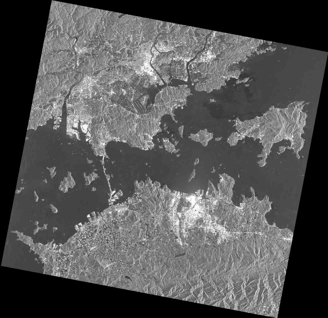
First we need to rewarp the .dat format to GeoTIFF which also applies the included Ground Control Points (GCPs) to the image. The resulting GeoTIFF file is then geocoded in Lat-Long/WGS84:
- gdalinfo PASL1500911220116591001270049_ortho.dat
- gdalwarp PASL1500911220116591001270049_ortho.dat PASL1500911220116591001270049_ortho.tif
Now we can auto-generate a GRASS Location from the GeoTIFF:
- Start 'grass64 -wx' or from menu (graphical user interface)
- Select Location Wizard
- Define a good name for the Location, then Next
- Select the item "Read projection and datum terms from a georeferenced file", then select the newly created PASL1500911220116591001270049_ortho.tif file, Next.
- Now the location is generated and the region is set to the image dimensions (degree in this case)
- You will return to the GRASS entry screen and can open the new location. Still the data have to be imported.
When in GRASS, import the map and display it:
- import with File -> Import raster map -> Import raster data using GDAL (r.in.gdal) -> Select again PASL1500911220116591001270049_ortho.tif and define name for this map in GRASS, when finished close dialog window
- Add map to map tree in the layer manager, using the icon
 . It should be automatically displayed
 - Use the zoom tool
 in the map display manager to zoom Mount Fuji
 - You will not recognize much yet since a better color map has to be assigned
Optimize the color table to better see the pixels:
- Press the right mouse button on the PALSAR map in the layer manager and select "Select color table".
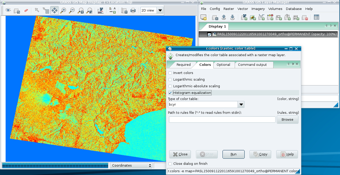
- In the "Required" tab the map name has to be selected; in the "Optional" tab select "Histogram equalization" and the "bcyr" color table. Click "Run" to generate the new color table. Then use the "Layer redraw" icon
 to see the updated map in the map display window.

Simple PALSAR image statistics:
- To calculate the image statistics (r.univar): in the menu, Raster -> Reports and Statistics -> Univariate raster statistics. Select the map (should be already there) and tick the checkbox "Calculate extended statistics" in the "optional" tab, then "Run". This takes a moment... Find the result in the "output command" tab. Check "mean" and "3rd quartile" and note the values down somewhere. In this example: mean: 352.068, 3rd quartile: 514 etc. Then close the dialog window.
- These values could be used to define a threshold filter in r.mapcalc.
Other PALSAR in GRASS GIS example
This example is based on sample data on the PALSAR web site (L1.5 GC product, L150FBS_GC):

Import:
 r.in.gdal PASL1500701140134440805020299_ortho.tif out=PASL1500701140134440805020299_ortho
 g.region rast=PASL1500701140134440805020299_ortho
Outlier reduction (only for visibility purposes!)
 r.univar PASL1500701140134440805020299_ortho
 # .. using 90% percentile:
 r.mapcalc "PASL1500701140134440805020299_ortho_filt  < 416.0, PASL1500701140134440805020299_ortho, null() )"
 r.colors PASL1500701140134440805020299_ortho_filt color=grey
 d.rast PASL1500701140134440805020299_ortho_filt
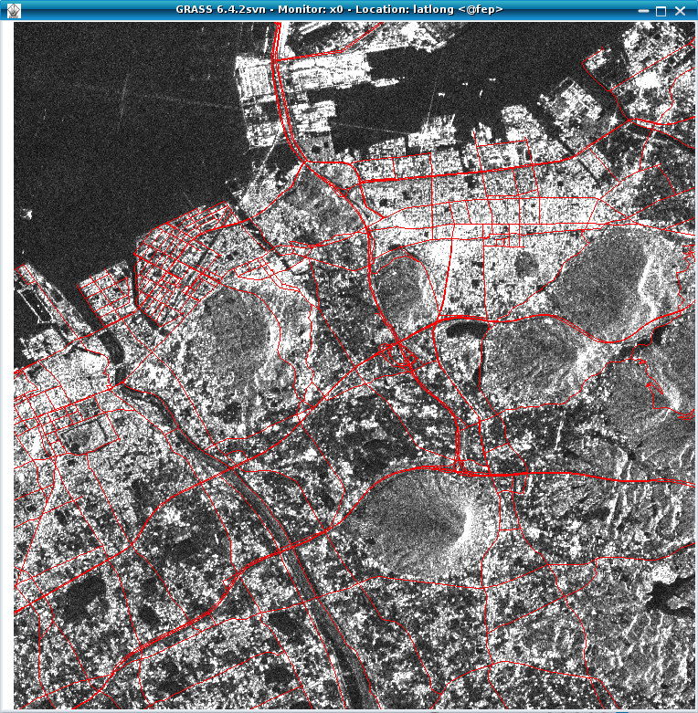
 d.vect osm_roads

The map shows nicely the fit of the circa 6m resolution PALSAR data and the OpenStreetMap vector lines (compare to Google Maps optical coverage).
Processing ALOS-PALSAR for Landcover Classification
Note: Original process was taken from an ASF MapReady and ENVI tutorial, the objective is to "port" the process using GRASS-GIS
- Pre-processing and image interpretation
- Conversion of raw ALOS-PALSAR mosaic image into GeoTIFF.
- Spatial subset
- DEM pre-processing
- Extracting Slope and Aspect from DEM
- Contrast stretching
- Edge enhancement - median and laplacian filter
- Speckle suppresion
- Antenna pattern correction
- Speckle filtering - lee, kuan, frost filters
- Supervised classification
- Conversion from aplitude to normalized radar data cross section
- Image slope/indidence angle correction
- Image classification
Sample data
- Palsar data download (various)
- RAT data download (various)
- ESA dataset package (Italy Earthquake, April 2009)
- PALSAR K & C Mosaic
You may want to get additionally some vector data, for example from Openstreetmap:
- http://download.geofabrik.de/osm/ (LatLong)
See also
- Introduction to Radar data processing
- RADAR and SAR Glossary
- CCRS Tutorial: Radar Remote Sensing (PDF)
- SAR Image Processing using GRASS (PDF ver1.1, Mar. 11, 2009; copy from http://www.safe.iis.u-tokyo.ac.jp/)