Using GRASS GIS through Python and tangible interfaces (workshop at FOSS4G NA 2016)

This is material for FOSS4G NA 2016 workshop *Using GRASS GIS through Python and tangible interfaces* held in Raleigh May 2, 2016 - 09:00 to 13:00. It was partially updated and used in classes at NCSU.
Learn about scripting, graphical and tangible (!) interfaces for GRASS GIS, the powerful desktop GIS and geoprocessing backend. We will start with the Python interface and finish with Tangible Landscape, a new tangible interface for GRASS GIS (see a webinar video). Python is the primary scripting language for GRASS GIS. We will demonstrate how to use Python to automate your geoprocessing workflows with GRASS GIS modules and develop custom algorithms using a Pythonic interface to access low level GRASS GIS library functions. We will also review several tips and tricks for parallelization. Tangible Landscape is an example of how the GRASS GIS Python API can be used to build new, cutting edge tools and advanced applications. Tangible Landscape is a collaborative 3D sketching tool which couples a 3D scanner, a projector and a physical 3D model with GRASS GIS. The workshop will be a truly hands-on experience – you will play with Tangible Landscape, using your hands to shape a sand model and drive geospatial processes.
Software: GRASS GIS 7
Data: Download complete North Carolina sample dataset.
GRASS GIS introduction
You need to create a GRASS database we will use for the tutorial. Please download the dataset for the workshop, noting where the files are located on your local directory. Now, create (unless you already have it) a directory named grassdata (GRASS database) in your home folder (or Documents), unzip the downloaded data into this directory. You should now have a Location nc_spm_08_grass7 in grassdata. Start GRASS GIS in Mapset user1.
GRASS GUI introduction
GRASS GIS Python API
Python Scripting library
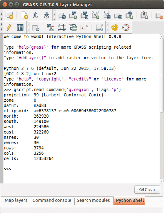
The GRASS GIS 7 Python Scripting Library provides functions to call GRASS modules within scripts as subprocesses. The most often used functions include:
- script.core.run_command(): most often used with modules which output raster/vector data where text output is not expected
- script.core.read_command(): used when we are interested in text output
- script.core.parse_command(): used with modules producing text output as key=value pair
- script.core.write_command(): for modules expecting text input from either standard input or file
Besides, this library provides several wrapper functions for often called modules.
Calling GRASS GIS modules
We will use GRASS GUI Python Shell to run the commands. For longer scripts, you can create a text file, save it into your current working directory and run it with python myscript.py from the GUI command console or terminal.
Tip: When copying Python code snippets to GUI Python shell, right click at the position and select Paste Plus in the context menu. Otherwise multiline code snippets won't work.
We start by importing GRASS GIS Python Scripting Library:
import grass.script as gs
Before running any GRASS raster modules, you need to set the computational region using g.region. In this example, we set the computational extent and resolution to the raster layer elevation.
gs.run_command('g.region', raster='elevation')
The run_command() function is the most commonly used one. Here, we apply the focal operation average (r.neighbors) to smooth the elevation raster layer. Note that the syntax is similar to bash syntax, just the flags are specified in a parameter.
gs.run_command('r.neighbors', input='elevation', output='elev_smoothed', method='average', flags='c')
If we run the Python commands from GUI Python console, we can use AddLayer to add the newly created layer:
AddLayer('elev_smoothed')
Calling GRASS GIS modules with textual input or output
Textual output from modules can be captured using the read_command() function.
gs.read_command('g.region', flags='p')
gs.read_command('r.univar', map='elev_smoothed', flags='g')
Certain modules can produce output in key-value format which is enabled by the -g flag. The parse_command() function automatically parses this output and returns a dictionary. In this example, we call g.proj to display the projection parameters of the actual location.
gs.parse_command('g.proj', flags='g')
For comparison, below is the same example, but using the read_command() function.
gs.read_command('g.proj', flags='g')
Certain modules require the text input be in a file or provided as standard input. Using the write_command() function we can conveniently pass the string to the module. Here, we are creating a new vector with one point with v.in.ascii. Note that stdin parameter is not used as a module parameter, but its content is passed as standard input to the subprocess.
gs.write_command('v.in.ascii', input='-', stdin='%s|%s' % (635818, 221342), output='point')
If we run the Python commands from GUI Python console, we can use AddLayer to add the newly created layer:
AddLayer('point')
Convenient wrapper functions
Some modules have wrapper functions to simplify frequent tasks. For example we can obtain the information about a raster layer with raster_info which is a wrapper of r.info, or a vector layer with script.vector.vector_info().
gs.raster_info('elevation')
gs.vector_info('point')
Another example is using script.raster.mapcalc() for raster algebra:
gs.mapcalc("elev_strip = if(elevation > 100 && elevation < 125, elevation, null())")
gs.read_command('r.univar', map='elev_strip', flags='g')
Function script.core.region() is a convenient way to retrieve the current region settings (i.e., computational region). It returns a dictionary with values converted to appropriate types (floats and ints).
region = gs.region()
print region
# cell area in map units (in projected Locations)
region['nsres'] * region['ewres']
We can list data stored in a GRASS GIS location with g.list wrappers. With script.core.list_grouped(), the map layers are grouped by mapsets (in this example, raster layers):
gs.list_grouped(type=['raster'])
gs.list_grouped(type=['raster'], pattern="landuse*")
Here is an example of a different g.list wrapper script.core.list_pairs() which structures the output as list of pairs (name, mapset). We obtain current mapset with g.gisenv wrapper.
current_mapset = gs.gisenv()['MAPSET']
gs.list_pairs('raster', mapset=current_mapset)
Exercise
Export all raster layers from your mapset with a name prefix "elev_*" as GeoTiff (see r.out.gdal). Don't forget to set the current region (g.region) for each map in order to match the individual exported raster layer extents and resolutions since they may differ from each other.
PyGRASS
PyGRASS is a library originally developed during the Google Summer of Code 2012. PyGRASS library adds two main functionalities:
- Python interface through the ctypes binding of the C API of GRASS, to read and write natively GRASS GIS 7 data structures,
- GRASS GIS module interface using objects to check the parameters and execute the respective modules.
For further discussion about the implementation ideas and performance are presented in the article: Zambelli, P.; Gebbert, S.; Ciolli, M. Pygrass: An Object Oriented Python Application Programming Interface (API) for Geographic Resources Analysis Support System (GRASS) Geographic Information System (GIS). ISPRS Int. J. Geo-Inf. 2013, 2, 201-219.
Standard scripting with GRASS modules in Python may sometime seem discouraging especially when you have to do conceptually simple things like iterate over vector features or raster rows/columns. Using the C API (most of GRASS GIS is written in C), all this is much more simple since you can directly work on GRASS GIS data and do just what you need to do. However, you perhaps want to stick to Python. Here, the PyGRASS library introduced several objects that allow to interact directly with the data using the underlying C API of GRASS GIS.
Working with vector data (see manual page)
Create a new vector map. Import the necessary classes:
from grass.pygrass.vector import VectorTopo
from grass.pygrass.vector.geometry import Point
Create an instance of a vector map:
my_points = VectorTopo('my_points')
Open the map in write mode:
my_points.open(mode='w')
Create some vector geometry features, like two points:
point1 = Point(635818.8, 221342.4)
point2 = Point(633627.7, 227050.2)
Add the above two points to the new vector map:
my_points.write(point1)
my_points.write(point2)
Finally close the vector map:
my_points.close()
Display the newly created vector (from GUI Python Shell):
AddLayer('my_points')
Now do the same thing using the context manager syntax and set also the attribute table:
# Define the columns of the new vector map
cols = [(u'cat',       'INTEGER PRIMARY KEY'),
        (u'name',      'TEXT')]

with VectorTopo('my_points', mode='w', tab_cols=cols, overwrite=True) as my_points:
    # save the point and the attribute
    my_points.write(point1, ('pub', ))
    my_points.write(point2, ('restaurant', ))
    # save the changes to the database
    my_points.table.conn.commit()
Note: we don't need to close the vector map because it is already closed by the context manager.
Go to Layer Manager, right click on 'my_points' and Show attribute data.
Read an existing vector map:
with VectorTopo('my_points', mode='r') as points:
    for point in points:
        print(point, point.attrs['name'])
Working with raster data (see manual page)
Create a new raster map and derive it's new values from elevation raster. Import the necessary classes:
from grass.pygrass.raster import RasterRow
Open the existing raster in read mode and print first 5 values of the first row (indices from S to N):
elev = RasterRow('elevation')
print elev.exist()
print elev.mapset
elev.open('r')
print elev[0][:5]
elev.close()
Create a new raster and write value 1 for cells with elevation < 120 and 0 otherwise:
new = RasterRow('new')
new.open('w', overwrite=True)
for row in elev:
    new.put_row(row < 120)
new.close()
print new.exist()
Query old and new raster maps:
from grass.pygrass.vector import geometry

new.open('r')
elev.open('r')
poi1 = geometry.Point(632942, 225757)
poi2 = geometry.Point(641780, 217455)
print elev.get_value(poi1), new.get_value(poi1)
print elev.get_value(poi2), new.get_value(poi2)
new.close()
elev.close()
For more examples of using PyGRASS, please look at How to write a Python GRASS GIS 7 addon workshop from FOSS4G-Europe 2015 and additional tutorials can be found on a PyGRASS wiki page.
Parallelization examples
A simple way to execute several modules in parallel (developed by Sören Gebbert) is the ParallelModuleQueue class. The basic idea is to create a queue with all the modules that must be execute in parallel. The ParallelModuleQueue class is based on the Module class of the pygrass library, here is a small example for computation of solar irradiance during day:
from copy import deepcopy
from grass.pygrass.modules import Module, ParallelModuleQueue

def main(elevation):
    # compute slope and aspect for r.sun
    Module('r.slope.aspect', elevation=elevation, aspect='aspect', slope='slope', overwrite=True)
    # initialize an empty queue and list
    queue = ParallelModuleQueue(nprocs=4)
    sun_name = 'sun_{}'
    # set computational region
    Module('g.region', raster=elevation)
    # initialize a module instance with shared inputs
    sun = Module('r.sun', elevation=elevation, slope='slope', aspect='aspect',
                 beam_rad='beam', step=1, day=123, run_=False, overwrite=True)

    for t in range(6, 22):
        # create a copy of the module and set the remaining parameters
        print t
        m = deepcopy(sun)(beam_rad=sun_name.format(t), time=t)
        queue.put(m)
    queue.wait()

    # set color table
    Module('r.colors', map=[sun_name.format(t) for t in range(6, 22)], color='grey', flags='e')

if __name__ == '__main__':
    elevation = 'elev_lid792_1m'
    main(elevation)
This simple parallel implementation uses Python class Pool:
from multiprocessing import Pool
import grass.script as gs

def rsun(params):
    gs.run_command('r.sun', **params)

def main(elevation):
    parameters = []
    sun_name = 'sun_{}'
    for t in range(6, 22):
        params = dict(elevation=elevation, slope='slope', aspect='aspect',
                      step=1, day=123, beam_rad=sun_name.format(t), time=t, overwrite=True)
        parameters.append(params)
    pool = Pool(4)
    p = pool.map_async(rsun, parameters)
    p.get()

if __name__ == '__main__':
    elevation = 'elev_lid792_1m'
    main(elevation)
This example shows parallelization by splitting computation into tiles using GridModule:
import grass.script as gs
from grass.pygrass.modules.grid import GridModule

def main(elevation):
    region = gs.region()
    width = region['cols'] // 2 + 1
    height = region['rows'] // 2 + 1

    grd = GridModule('r.slope.aspect', elevation=elevation, slope='slope',
                     debug=False, width=width, height=height,
                     overlap=10, processes=4, overwrite=True)
    grd.run()

if __name__ == '__main__':
    elevation = 'elevation'
    gs.run_command('g.region', raster=elevation)
    main(elevation)
Tangible Landscape
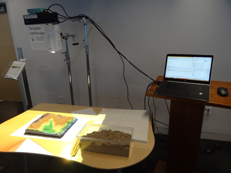
A brief introduction to Tangible Landscape
Tangible Landscape is a collaborative modeling environment for analysis of terrain changes. We couple a scanner, projector and a physical 3D model with GRASS GIS. We can analyze the impact of terrain changes by capturing the changes on the model, bringing them into the GIS, performing desired analysis or simulation and projecting the results back on the model in real-time. Tangible Landscape, as an easy-to-use 3D sketching tool, enables rapid design and scenarios testing for people with different backgrounds and computer knowledge, as well as support for decision-making process.
Tangible Landscape has been used for a variety of applications supported by the extensive set of geospatial analysis and modeling tools available in GRASS GIS. We have explored how dune breaches affect the extent of coastal flooding, the impact of different building configurations on cast shadows and solar energy potential, and the effectiveness of various landscape designs for controlling runoff and erosion. Have a look at our [tangible-landscape.github.io/ website], book, and Youtube channel.
The software is free and open source and you can download it and use it in your own setup of Tangible Landscape.
Presentation here
Running examples
We will use a repository on GitHub to collect code samples participants and then run them in the Tangible Landscape environment (we used Titanpad during the 2016 workshop and codeshare in a 2019 class and switched to GitHub repositories such as these: 2020, 2021). Whenever a scanning cycle is complete, a specified Python file is imported and all analyses in that file are computed. Analyses are organized into functions with defined interface - each function has to start with run_. Input parameter scanned_elev is the scanned raster (our DEM) and env is the environment which needs to be passed to individual subprocesses to correctly handle the region of the analysis.
Since participants will develop and test the analyses on their computers before we apply them to Tangible Landscape, we add here the 'main' function with predefined parameters and participants will run it as a script.
import grass.script as gs

def run_slope(scanned_elev, env, **kwargs):
    # compute the analysis
    gs.run_command('r.slope.aspect', ..., env=env)

if __name__ == '__main__':
    import os
    os.environ['GRASS_OVERWRITE'] = '1'
    elevation = 'elev_lid792_1m'
    run_slope(scanned_elev=elevation, env=None)
We will run the scripts from Simple Python Editor (Python tab -> Simple editor). Alternatively, scripts can be run from terminal or GUI command console:
python /path/to/my/script.py
On Windows the path will look differently, for example:
python C:\Users\yourname\path\to\my\script.py
Make sure you set computational region to match your DEM. We will use raster DEM elev_lid792_1m from the sample dataset.
g.region raster=elev_lid792_1m -p
Here follow some basic examples of geospatial analyses we can do with Tangible Landscape. At the end of this section you can find additional tasks, some of them combining multiple analyses.
Modeling topography
Computing slope
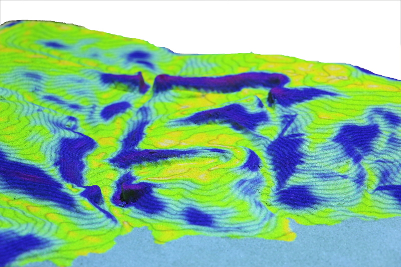
Basic example how we can compute topographic slope in degrees:
import grass.script as gs

def run_slope(scanned_elev, env, **kwargs):
    gs.run_command('r.slope.aspect', elevation=scanned_elev, slope='slope', env=env)

if __name__ == '__main__':
    elevation = 'elev_lid792_1m'
    env = None
    run_slope(scanned_elev=elevation, env=env)
We can compute slope in percent and reclassify the values into discrete intervals:
def run_slope(scanned_elev, env, **kwargs):
    gs.run_command('r.slope.aspect', elevation=scanned_elev, slope='slope',
                        format='percent', env=env)
    # reclassify using rules passed as a string to standard input
    # 0:2:1 means reclassify interval 0 to 2 percent of slope to category 1
    rules = ['0:2:1', '2:5:2', '5:8:3', '8:15:4', '15:30:5', '30:*:6']
    gs.write_command('r.recode', input='slope', output='slope_class',
                          rules='-', stdin='\n'.join(rules), env=env)
    # set new color table: green - yellow - red
    gs.run_command('r.colors', map='slope_class', color='gyr', env=env)
Curvatures
Explore concavity/convexity of terrain with curvatures computed by r.param.scale:
def run_curvatures(scanned_elev, env, **kwargs):
    gs.run_command('r.param.scale', input=scanned_elev, output='profile_curv',
                   method='profc', size=11, env=env)
    gs.run_command('r.param.scale', input=scanned_elev, output='tangential_curv',
                   method='crosc', size=11, env=env)
    gs.run_command('r.colors', map=['profile_curv', 'tangential_curv'], color='curvature', env=env)
Change window size and see how it influences the result.
Landform identification
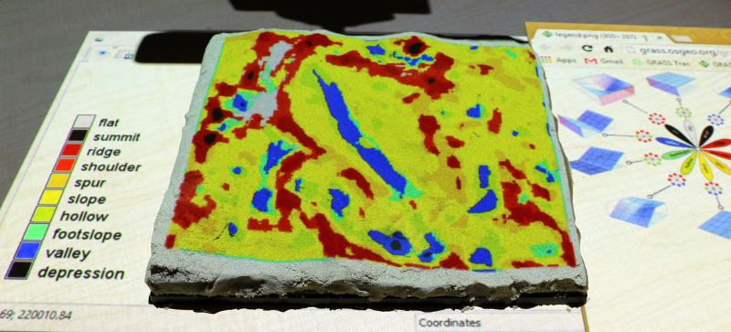
There are 2 different methods for landform (ridge, valley, ...) identification in GRASS GIS. First one is implemented in r.param.scale and uses curvatures. The second is implemented in an addon r.geomorphon which uses multiscale line-of-sight approach. This addon can be installed from GUI command line:
g.extension r.geomorphon
or follow this tutorial.
def run_curvatures(scanned_elev, env, **kwargs):
    gs.run_command('r.param.scale', input=scanned_elev, output='landforms1',
                   method='feature', size=10, env=env)
    gs.run_command('r.geomorphon', elevation=scanned_elev, forms='landforms2',
                   search=16, skip=6, env=env)
Building model based on difference raster
When building a model by hands based on a defined DEM, we can compute the difference between the scanned model and the original DEM. By color-coding the difference, we can see where to add sand or remove it.
If you are running this outside of Tangible Landscape, you can generate a raster (our hypothetical pile of sand) and compute the difference. In this example we also vertically rescale and translate the scanned raster to match the original DEM using r.regression.line.
import grass.script as gs

def run_difference(real_elev, scanned_elev, env, **kwargs):
    regression_params = gs.parse_command('r.regression.line', flags='g', mapx=scanned_elev, mapy=real_elev, env=env)
    gs.mapcalc('{regression} = {a} + {b} * {before}'.format(a=regression_params['a'], b=regression_params['b'],
                                                            before=scanned_elev, regression='regression'), env=env)
    gs.mapcalc('{difference} = {regression} - {after}'.format(regression='regression', after=real_elev, difference='diff'), env=env)
    gs.write_command('r.colors', map='diff', rules='-', stdin="-100 black\n-20 red\n0 white\n20 blue\n100 black", env=env)

if __name__ == '__main__':
    elevation = 'elev_lid792_1m'
    sand_pile = 'sand_pile'
    env = None
    gs.run_command('r.surf.fractal', output=sand_pile)
    run_difference(real_elev=elevation, scanned_elev=sand_pile, env=env)
Hydrology
Flooding with r.lake
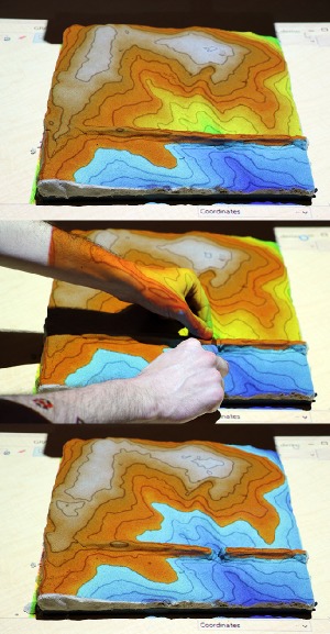
Module r.lake fills a lake to a target water level from a given start point or seed raster. The resulting raster map contains cells with values representing lake depth and NULL for all other cells beyond the lake.
Example showing basic usage:
def run_lake(scanned_elev, env, **kwargs):
    coordinates = [638830, 220150]
    gs.run_command('r.lake', elevation=scanned_elev, lake='output_lake',
                   coordinates=coordinates, water_level=120, env=env)
Create a lake where water level is relative to the altitude of the seed cell. Use function script.raster.raster_what() to obtain the elevation value of the DEM and create a lake with water level being for example 5 m higher.
def run_lake(scanned_elev, env, **kwargs):
    coordinates = [638830, 220150]
    res = gs.raster_what(map=scanned_elev, coord=[coordinates])
    elev_value = float(res[0][scanned_elev]['value'])
    gs.run_command('r.lake', elevation=scanned_elev, lake='output_lake',
                   coordinates=coordinates, water_level=elev_value + 5, env=env)
Flow accumulation and watersheds
We can derive watersheds and flow accumulation using module r.watershed in one command:
def run_hydro(scanned_elev, env, **kwargs):
    gs.run_command('r.watershed', elevation=scanned_elev, accumulation='flow_accum',
                   basin='watersheds', threshold=1000, flags='a', env=env)
Compute average slope value for each watershed. To do that use zonal statistics using r.stats.zonal:
def run_watershed_slope(scanned_elev, env, **kwargs):
    gs.run_command('r.watershed', elevation=scanned_elev, accumulation='flow_accum',
                   basin='watersheds', threshold=1000, env=env)
    gs.run_command('r.slope.aspect', elevation=scanned_elev, slope='slope', env=env)
    gs.run_command('r.stats.zonal', base='watersheds', cover='slope', method='average',
                   output='watersheds_slope', env=env)
    gs.run_command('r.colors', map='watersheds_slope', color='bgyr', env=env)
Depression filling
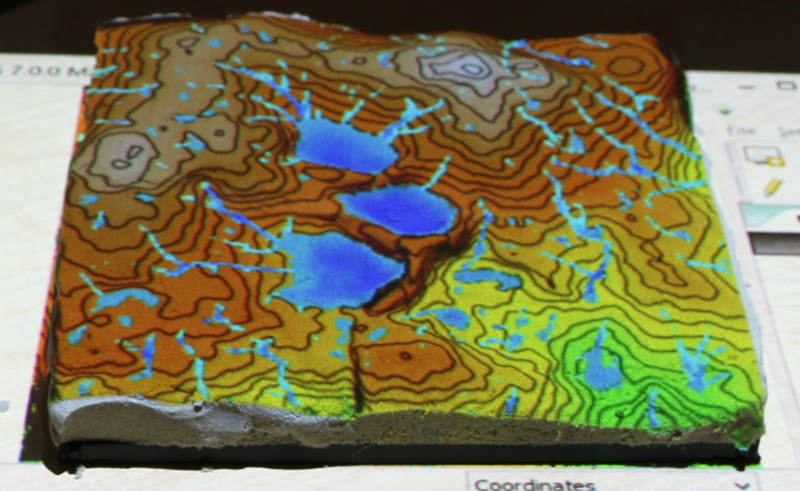
We will use depression filling algorithm implemented in r.fill.dir not as preprocessing step for flow accumulation analysis, but for creating ponds. Because depressions are often nested, we will run depression filling several times:
def run_ponds(scanned_elev, env, **kwargs):
    repeat = 2
    input_dem = scanned_elev
    output = "tmp_filldir"
    for i in range(repeat):
        gs.run_command('r.fill.dir', input=input_dem, output=output, direction="tmp_dir", env=env)
        input_dem = output
    # filter depression deeper than 0.1 m to
    gs.mapcalc('{new} = if({out} - {scan} > 0.1, {out} - {scan}, null())'.format(new='ponds', out=output,
                                                                                 scan=scanned_elev), env=env)
    gs.write_command('r.colors', map='ponds', rules='-', stdin='0% aqua\n100% blue', env=env)
Overland water flow simulation
Module r.sim.water is an overland flow hydrology simulation using path sampling method.
def run_waterflow(scanned_elev, env, **kwargs):
    # first we need to compute x- and y-derivatives
    gs.run_command('r.slope.aspect', elevation=scanned_elev, dx='scan_dx', dy='scan_dy', env=env)
    gs.run_command('r.sim.water', elevation=scanned_elev, dx='scan_dx', dy='scan_dy',
                   rain_value=150, depth='flow', env=env)
Erosion modeling
Landscape potential for soil erosion and deposition can be estimated and mapped using Unit Stream Power Based Erosion Deposition model (USPED). In this example we will use uniform land cover (c factor) and soil erodibility (K factor). Install addon r.divergence using g.extension.
def run_usped(scanned_elev, env, **kwargs):
    gs.run_command('r.slope.aspect', elevation=scanned_elev, slope='slope', aspect='aspect', env=env)
    gs.run_command('r.watershed', elevation=scanned_elev, accumulation='flow_accum', threshold=1000, flags='a', env=env)
    # topographic sediment transport factor
    resolution = gs.region()['nsres']
    gs.mapcalc("sflowtopo = pow(flow_accum * {res}.,1.3) * pow(sin(slope),1.2)".format(res=resolution), env=env)
    # compute sediment flow by combining the rainfall, soil and land cover factors with the topographic sediment transport factor. We use a constant value of 270 for rainfall intensity factor
    gs.mapcalc("sedflow = 270. * {k_factor} * {c_factor} * sflowtopo".format(c_factor=0.05, k_factor=0.1), env=env)
    # compute divergence of sediment flow
    gs.run_command('r.divergence', magnitude='sedflow', direction='aspect', output='erosion_deposition', env=env)
    colors = ['0% 100:0:100', '-100 magenta', '-10 red', '-1 orange', '-0.1 yellow', '0 200:255:200',
              '0.1 cyan', '1 aqua', '10 blue', '100 0:0:100', '100% black']
    gs.write_command('r.colors', map='erosion_deposition',  rules='-', stdin='\n'.join(colors), env=env)
Solar radiation and shades
We will first compute solar irradiation (daily radiation sum in Wh/m2.day) for a given day using r.sun:
def run_solar_radiation(scanned_elev, env, **kwargs):
    # convert date to day of year
    import datetime
    doy = datetime.datetime(2016, 5, 2).timetuple().tm_yday
    # precompute slope and aspect
    gs.run_command('r.slope.aspect', elevation=scanned_elev, slope='slope', aspect='aspect', env=env)
    gs.run_command('r.sun', elevation=scanned_elev, slope='slope', aspect='aspect', beam_rad='beam', step=1, day=doy, env=env)
    gs.run_command('r.colors', map='beam', color='grey', flags='e')
Then we can also compute solar irradiance (W/m2) for a given day and hour (in local solar time) and extract the shades cast by topography:
def run_solar_radiance(scanned_elev, env, **kwargs):
    # convert date to day of year
    import datetime
    doy = datetime.datetime(2016, 5, 2).timetuple().tm_yday
    # precompute slope and aspect
    gs.run_command('r.slope.aspect', elevation=scanned_elev, slope='slope', aspect='aspect', env=env)
    gs.run_command('r.sun', elevation=scanned_elev, slope='slope', aspect='aspect', beam_rad='beam', day=doy, time=8, env=env)
    # extract shade and set color to black and white
    gs.mapcalc("shade = if(beam == 0, 0, 1)", env=env)
    gs.run_command('r.colors', map='beam', color='grey')
Visibility analysis
First example shows computing viewshed (visibility) from a given coordinate:
def run_viewshed(scanned_elev, env, **kwargs):
    coordinates = [638830, 220150]
    gs.run_command('r.viewshed', input=scanned_elev, output='viewshed', coordinates=coordinates, observer_elevation=1.75, flags='b', env=env)
    gs.run_command('r.colors', map='viewshed', color='grey')
Cost surface and least cost path
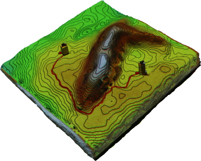
This example shows least cost path analysis with slope as cost. Coordinates will be provided by Tangible Landscape. The resulting path will go through flat areas.
import grass.script as gs
def LCP(elevation, start_coordinate, end_coordinate, env):
    gs.run_command('r.slope.aspect', elevation=scanned_elev, slope='slope', env=env)
    gs.run_command('r.cost', input='slope', output='cost', start_coordinates=start_coordinate,
                   outdir='outdir', flags='k', env=env)
    gs.run_command('r.colors', map='cost', color='gyr', env=env)
    gs.run_command('r.drain', input='cost', output='drain', direction='outdir',
                   drain='drain', flags='d', start_coordinates=end_coordinate, env=env)

if __name__ == '__main__':
    elevation = 'elev_lid792_1m'
    env = None
    start = [638469, 220070]
    end = [638928, 220472]
    LCP(elevation, start, end, env)
Additional tasks
- Compute topographic index using r.topidx.
- Compute topographic aspect (slope orientation) using r.slope.aspect and reclassify it into 8 main directions.
- Show areas with concave profile and tangential curvature (concave forms have negative curvature).
- Derive peaks using either r.geomorphon or r.param.scale and convert them to points (using r.to.vect and v.to.points). From each of those points compute visibility with observer height of your choice a derive a cumulative viewshed layer where the value of each cell represents the number of peaks the cell is visible from (use r.series).
- Find a least cost path between 2 points (for example from x=638360, y=220030 to x=638888, y=220388) where cost is defined as topographic index (trying avoid areas). Use r.topidx.
- Compute erosion with spatially variable landcover and soil erodibility (use rasters cfactorbare_1m and soils_Kfactor from the provided dataset). Reclassify the result into 7 classes based on severity of erosion and deposition:
-120000.:-10:1:1
-10.:-5.:2:2
-5.:-0.1:3:3
-0.1:0.1:4:4
0.1:5.:5:5
5.:10.:6:6
10.:150000.:7:7