Analytical data visualizations at ICC 2017

This is material for two sessions at the ICC 2017 SDI-Open (Spatial data infrastructures, standards, open source and open data for geospatial) workshop called Analytical data visualizations with GRASS GIS and Blender and Mapping open data with open source geospatial tools held in Washington, DC, July 1-2, 2017. These two sessions introduce GRASS GIS and Blender, example of their processing capabilities and visualization techniques. Participants interactively visualize open data and design maps with several open source geospatial tools including Tangible Landscape system.
Authors: Vaclav Petras, Anna Petrasova, Payam Tabrizian, Brendan Harmon, and Helena Mitasova
Testing and review: Garrett Millar
We start the workshop with a presentation about the overview of geospatial tools used in this workshop.
Note: Screenshots of GUI may be outdated, however the rest of the tutorial is updated to work with GRASS GIS 7.8.
Data
Prepared data
Workshop dataset contains:
- digital surface model (1m resolution) derived from publicly available North Carolina Flood Plain Mapping lidar
- orthophoto (0.5m resolution) from USGS
Download OpenStreetMap data
We will use overpass turbo (web-based data filtering tool) to create and run Overpass API queries to obtain OpenStreetMap data.
You can use Wizard to create simple queries on the currently zoomed extent. For example, zoom to a small area and paste this into the Wizard and run the query:
highway=* and type:way
The query was built in the editor and ran so you can now see the results in a map.
Now, paste this query in the editor window:
[out:json][timeout:25];
// gather results
(
  // query part for: "highway=*"
  way["highway"](35.76599,-78.66249,35.77230,-78.65261);
);
// print results
out body;
>;
out skel qt;
It finds roads in our study area. When you run the query, the roads appear on the map and we can export them as GeoJSON (Export - Data - as GeoJSON). Name the vector file roads.geojson.
Now let's also download all building footprints and again export them as GeoJSON. Name the vector file buildings.geojson.
[out:json][timeout:25];
// gather results
(
  // query part for: "building=*"
  way["building"](35.76599,-78.66249,35.77260,-78.65261);
  relation["building"](35.76599,-78.66249,35.77260,-78.65261);
);
// print results
out body;
>;
out skel qt;
In the next steps we will import this data into GRASS GIS.
Session 1: Introduction to GRASS GIS
Here we provide an overview of GRASS GIS. For this exercise it's not necessary to have a full understanding of how to use GRASS GIS. However, you will need to know how to place your data in the correct GRASS GIS database directory, as well as some basic GRASS functionality.
Structure of the GRASS GIS Spatial Database
GRASS uses unique database terminology and structure (GRASS GIS Spatial Database) that are important to understand for working in GRASS GIS efficiently. You will create a new location and import the required data into that location. In the following we review important terminology and give step by step directions on how to download and place your data in the correct place.
- A GRASS GIS Spatial Database (GRASS database) consists of directory with specific Locations (projects) where data (data layers/maps) are stored.
- Location is a directory with data related to one geographic location or a project. All data within one Location has the same coordinate reference system.
- Mapset is a collection of maps within Location, containing data related to a specific task, user or a smaller project.
-
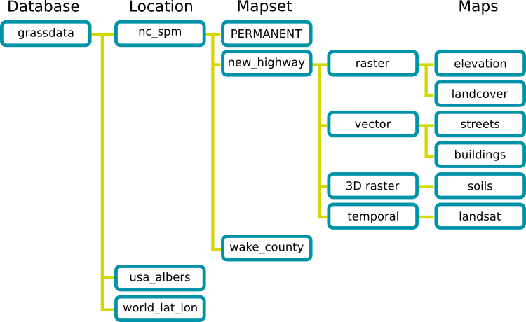
GRASS GIS Spatial Database structure

Creating a GRASS database for the tutorial
Start GRASS GIS, a start-up screen should appear. Unless you already have a directory called grassdata in your Documents directory (on MS Windows) or in your home directory (on Linux), create one. You can use the Browse button and the dialog in the GRASS GIS start up screen to do that.
We will create a new location for our project with CRS (coordinate reference system) NC State Plane Meters with EPSG code 3358. Open Location Wizard with button New in the left part of the welcome screen. Select a name for the new location, select EPSG method and code 3358. When the wizard is finished, the new location will be listed on the start-up screen. Select the new location and mapset PERMANENT and press Start GRASS session.
-
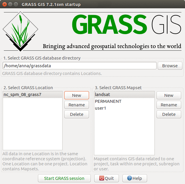
GRASS GIS 7.2 startup dialog
-
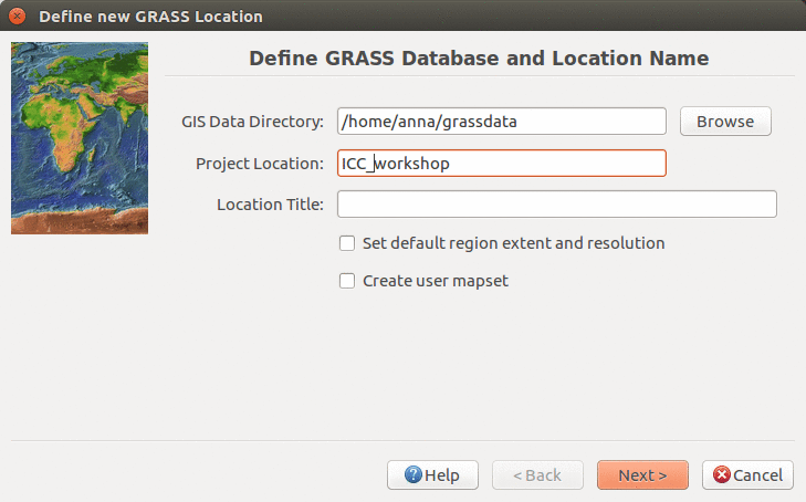
Start Location Wizard and type the new location's name
-
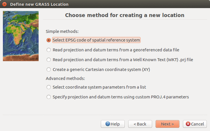
Select method for describing CRS
-
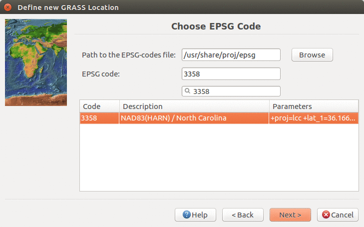
Find and select EPSG 3358
-
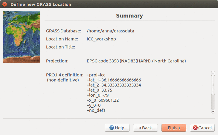
Review summary page and confirm


Current working directory
A current working directory is a concept which is separate from the GRASS database, location and mapset discussed above. The current working directory is a directory (also called folder) where any program (no just GRASS GIS) writes and reads files unless a path to the file is provided. When using GRASS GIS GUI, the current working directory is usually not used. However, when using command line or doing scripting, the current working directory is important.
Change your current working directory to some place where you have read and write permissions. For example, you can create a directory ICC in the Documents. The current working directory can be changed from the GUI using Settings → GRASS working environment → Change working directory or from the Console using the cd command.
Importing data

In this step we import the provided data into GRASS GIS. In menu File - Import raster data select Common formats import and in the dialog browse to find dsm.tif and click button Import. Repeat for raster file ground.tif and ortho.tif.
Similarly, go to File - Import vector data - Common formats import and import files roads.geojson and buildings.geojson. Note that in this case we need to change the output name from default OGRGeoJSON to roads and buildings, respectively. This vector data has different CRS, so a dialog informing you about the need to reproject the data appears and we confirm it.
All the imported layers should be added to GUI, if not, add them manually (see below).
Displaying and exploring data
The GUI interface allows you to display raster and vector data as well as navigate through zooming in and out. More advanced exploration and visualization is also possible using, e.g., queries and adding legend. The screenshots below depicts how you can add different map layers (left) and display the metadata of your data layers.
-
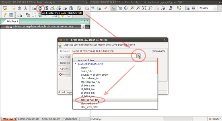
Add raster map layer
-
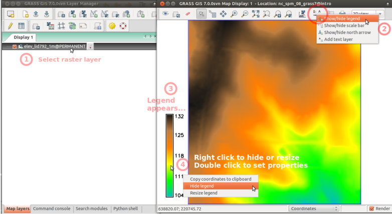
Add raster legend
-
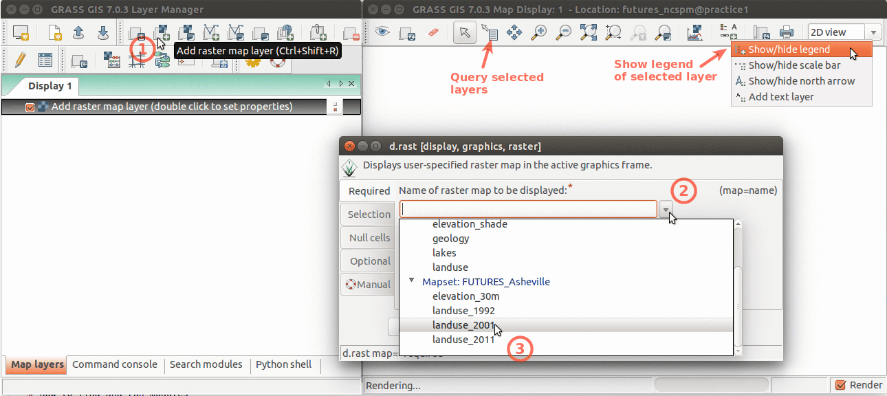
Layer Manager and Map Display overview. Annotations show how to add raster layer, query, add legend.
-
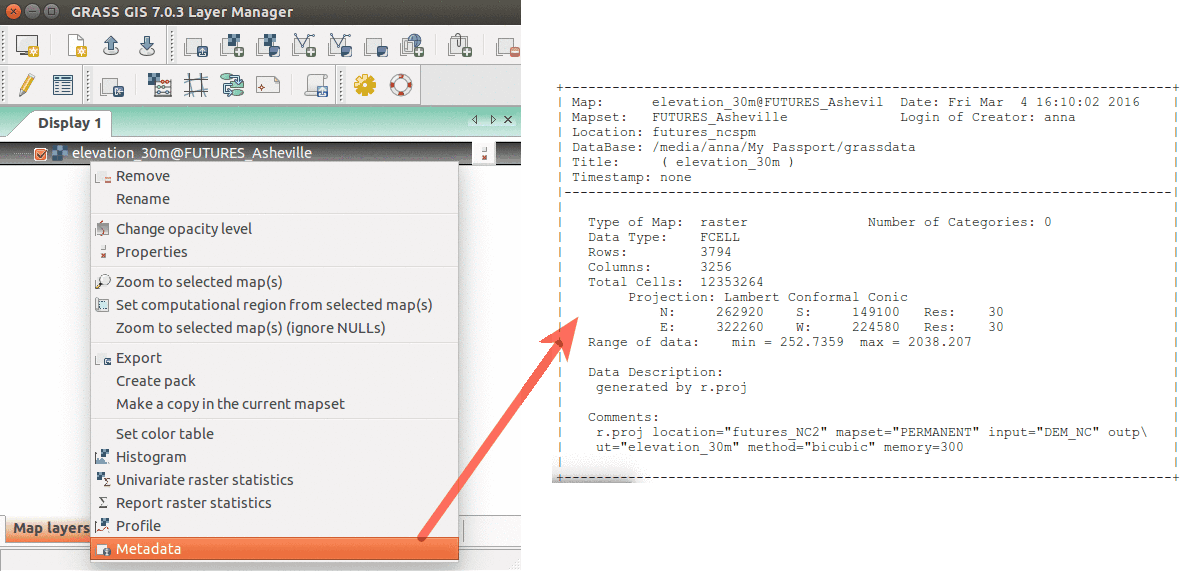
Show raster map metadata by right clicking on layer


GRASS GIS modules overview
One of the advantages of GRASS is the diversity and number of modules that let you analyze all manners of spatial and temporal data. GRASS GIS has over 500 different modules in the core distribution and over 300 addon modules that can be used to prepare and analyze data.
GRASS functionality is available through modules (tools, functions). Modules respect the following naming conventions:
| Prefix | Function | Example |
|---|---|---|
| r.* | raster processing | r.mapcalc: map algebra |
| v.* | vector processing | v.clean: topological cleaning |
| i.* | imagery processing | i.segment: object recognition |
| db.* | database management | db.select: select values from table |
| r3.* | 3D raster processing | r3.stats: 3D raster statistics |
| t.* | temporal data processing | t.rast.aggregate: temporal aggregation |
| g.* | general data management | g.rename: renames map |
| d.* | display | d.rast: display raster map |
These are the main groups of modules. There is a few more for specific purposes. Note also that some modules have multiple dots in their names. This often suggests further grouping. For example, modules staring with v.net. deal with vector network analysis.
The name of the module helps to understand its function, for example v.in.lidar starts with v so it deals with vector maps, the name follows with in which indicates that the module is for importing the data into GRASS GIS Spatial Database and finally lidar indicates that it deals with lidar point clouds.
Finding and running a module
To find a module for your analysis, type the term into the search box into the Modules tab in the Layer Manager, then keep pressing Enter until you find your module.
Alternatively, you can just browse through the module tree in the Modules tab. You can also browse through the main menu. For example, to find information about a raster map, use: Raster → Reports and statistics → Basic raster metadata.
If you already know the name of the module, you can just use it in the command line. The GUI offers a Console tab with command line specifically built for running GRASS GIS modules. If you type the module name there, you will get suggestions for automatic completion of the name. After pressing Enter, you will get GUI dialog for the module.
-
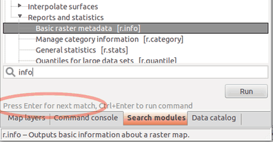
Search for a module in module tree (searches in names, descriptions and keywords)
-
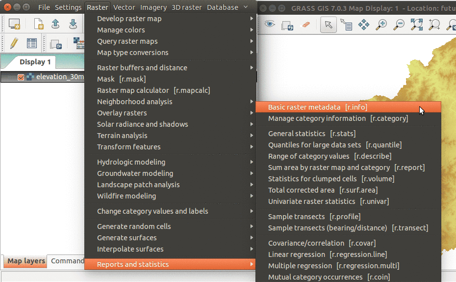
Modules can be also found in the main menu
-
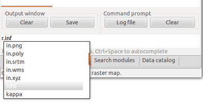
Automatic suggestions when typing name of the module: By typing prefix r. we make a list of modules starting with that prefix to show up.


You can also use the command line to run complete commands, i.e. module and list of parameters. These commands are what you usually find in the documentation or in this material. You can use them directly in the Console tab or you can use them as instructions how to fill the GUI dialog.
Command line vs. GUI interface

GRASS modules can be executed either through a GUI or command line interface. The GUI offers a user-friendly approach to executing modules where the user can navigate to data layers that they would like to analyze and modify processing options with simple check boxes. The GUI also offers an easily accessible manual on how to execute a model. The command line interface allows users to execute a module using command prompts specific to that module. This is handy when you are running similar analyses with minor modification or are familiar with the module commands for quick efficient processing. In this workshop we provide module prompts that can be copied and pasted into the command line for our workflow, but you can use both the GUI and command line interface depending on personal preference. Look how GUI and command line interface represent the same tool.
The same analysis can be done using the following command:
r.neighbors -c input=elevation output=elev_smooth size=5
Conversely, you can fill the GUI dialog parameter by parameter when you have the command.
Computational region
Before we use a module to compute a new raster map, we must properly set the computational region. All raster computations will be performed in the specified extent and with the given resolution.
Computational region is an important raster concept in GRASS GIS. In GRASS a computational region can be set, subsetting larger extent data for quicker testing of analysis or analysis of specific regions based on administrative units. We provide a few points to keep in mind when using the computational region function:
- defined by region extent and raster resolution
- applies to all raster operations
- persists between GRASS sessions, can be different for different mapsets
- advantages: keeps your results consistent, avoid clipping, for computationally demanding tasks set region to smaller extent, check that your result is good and then set the computational region to the entire study area and rerun analysis
- run
g.region -por in menu Settings - Region - Display region to see current region settings
-
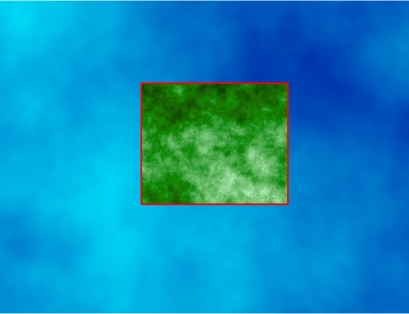
Computational region concept: A raster with large extent (blue) is displayed as well as another raster with smaller extent (green). The computational region (red) is now set to match the smaller raster, so all the computations are limited to the smaller raster extent even if the input is the larger raster. (Not shown on the image: Also the resolution, not only the extent, matches the resolution of the smaller raster.)
-
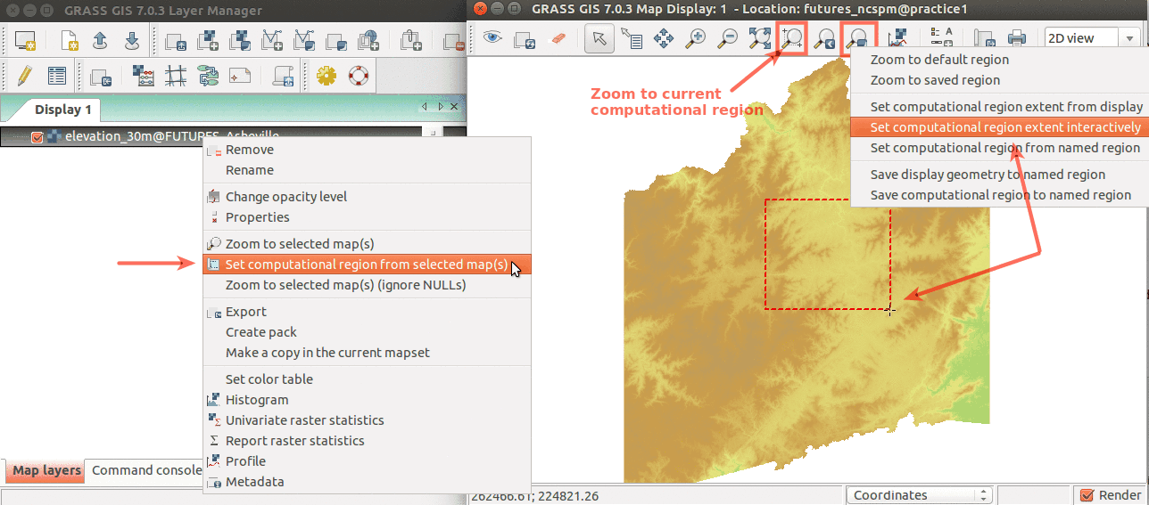
Simple ways to set computational region from GUI: On the left, set region to match raster map. On the right, select the highlighted option and then set region by drawing rectangle.
-
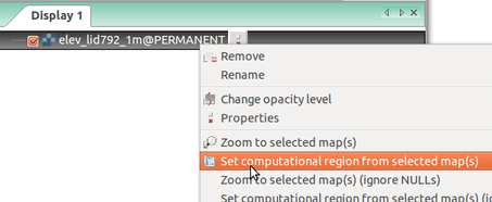
Set computational region (extent and resolution) to match a raster (Layers tab in the Layer Manager)


The numeric values of computational region can be checked using:
g.region -p
After executing the command you will get something like this:
north:      220750
south:      220000
west:       638300
east:       639000
nsres:      1
ewres:      1
rows:       750
cols:       700
cells:      525000
Computational region can be set using a raster map:
g.region raster=dsm -p
Running modules
Find the module for computing viewshed in the menu or the module tree under Raster → Terrain analysis → Visibility, or simply run r.viewshed from the Console.
r.viewshed input=dsm output=dsm_viewshed coordinates=640167,223907 observer_elevation=1.72 target_elevation=1 max_distance=400
3D view

We can explore our study area in 3D view (use image on the right if clarification is needed for below steps):
- Add raster dsm and uncheck or remove any other layers. Any layer in Layer Manager is interpreted as surface in 3D view.
- Switch to 3D view (in the right corner of Map Display).
- Adjust the view (perspective, height).
- In Data tab, set Fine mode resolution to 1 and set ortho as the color of the surface (the orthophoto is draped over the DSM).
- Go back to View tab and explore the different view directions using the green puck.
- Go again to Data tab and change color to viewshed raster computed in the previous steps.
- Go to Appearance tab and change the light conditions (lower the light height, change directions).
- When finished, switch back to 2D view.
Session 1: Introduction to scripting in GRASS GIS with Python
The simplest way to execute the Python code which uses GRASS GIS packages is to use Simple Python editor integrated in GRASS GIS (accessible from the toolbar or the Python tab in the Layer Manager). Another option is to write the Python code in your favorite plain text editor like Notepad++ (note that Python editors are plain text editors). Then run the script in GRASS GIS using the main menu File -> Launch script.
-
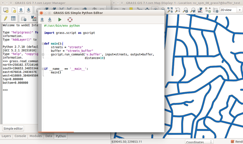
Simple Python Editor integrated in GRASS GIS (since version 7.2) with Python tab in the background which contains an interactive Python shell.
-
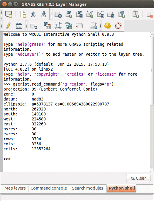
Python tab with an interactive Python shell


The GRASS GIS 7 Python Scripting Library provides functions to call GRASS modules within scripts as subprocesses. The most often used functions include:
- script.core.run_command(): used with modules which output raster/vector data where text output is not expected
- script.core.read_command(): used when we are interested in text output
- script.core.parse_command(): used with modules producing text output as key=value pair
- script.core.write_command(): for modules expecting text input from either standard input or file
We will use GRASS GUI Simple Python Editor to run the commands. You can open it from Python tab. For longer scripts, you can create a text file, save it into your current working directory and run it with python myscript.py from the GUI command console or terminal.
When you open Simple Python Editor, you find a short code snippet. It starts with importing GRASS GIS Python Scripting Library:
import grass.script as gs
In the main function we call g.region to see the current computational region settings:
gs.run_command('g.region', flags='p')
Note that the syntax is similar to bash syntax (g.region -p), only the flag is specified in a parameter. Now we can run the script by pressing the Run button in the toolbar. In Layer Manager we get the output of g.region.
Before running any GRASS raster modules, you need to set the computational region. In this example, we set the computational extent and resolution to the raster layer elevation. Replace the previous g.region command with the following line:
gs.run_command('g.region', raster='dsm')
The run_command() function is the most commonly used one. We will use it to compute viewshed using r.viewshed. Add the following line after g.region command:
gs.run_command('r.viewshed', input='dsm', output='python_viewshed', coordinates=(640645, 224035), overwrite=True)
Parameter overwrite is needed if we rerun the script and rewrite the raster.
Now let's look at how big the viewshed is by using
r.univar. Here we use parse_command to obtain the statistics as a Python dictionary
univar = gs.parse_command('r.univar', map='python_viewshed', flags='g')
print(univar['n'])
The printed result is the number of cells of the viewshed.
GRASS GIS Python Scripting Library also provides several wrapper functions for often called modules. List of convenient wrapper functions with examples includes:
- Raster metadata using script.raster.raster_info():
gs.raster_info('viewshed_python') - Vector metadata using script.vector.vector_info():
gs.vector_info('roads') - List raster data in current location using script.core.list_grouped():
gs.list_grouped(type=['raster']) - Get current computational region using script.core.region():
gs.region()
Here are two commands (to be executed in the Console) often used when working with scripts. First is setting the computational region. We can do that in a script, but it is better and more general to do it before executing the script (so that the script can be used with different computational region settings):
g.region raster=dsm
The second command is handy when we want to run the script again and again. In that case, we first need to remove the created raster maps, for example:
g.remove type=raster pattern="viewshed*"
The above command actually won't remove the maps, but it will inform you which it will remove if you provide the -f flag.
Session 1: Batch processing using Python
In this example, we will calculate the viewsheds along a road to simulate, in a simple way, what a driver would see. First we will prepare view points by running the modules directly through the GUI dialogs or in the Console. Then we will use Python to process all the created points.
First we extract only segments of road with name 'Umstead Drive' (use the code in the Console tab or use the GUI dialog):
v.extract input=roads where="name = 'Umstead Drive'" output=umstead_drive_segments
We will join the segments into one polyline using v.build.polylines
v.build.polylines input=umstead_drive_segments output=umstead_drive cats=first
Now we generate viewpoints in regular intervals along the line:
v.to.points input=umstead_drive type=line output=viewpoints dmax=50
We compute viewshed from each point using a Python script. We will use the difference between the DSM and ground elevation to filter out points that happen to lie on some vegetation covering the road. This is to avoid computing viewsheds from the top of a tree, which would significantly distort viewshed size.
 r.mapcalc "diff = dsm - ground"
 r.colors map=diff color=differences
From these viewsheds we can then easily compute Cumulative viewshed (how much a place is visible). For that we will use module r.series, which overlays the viewshed rasters and computes how many times each cell is visible in all the rasters.
Copy the following code into Python Simple Editor (be sure to overwrite any already existing code) and press Run button.
#!/usr/bin/env python3

import grass.script as gs

def main():
    # obtain the coordinates of viewpoints
    viewpoints = gs.read_command('v.out.ascii', input='viewpoints',
                                 separator='comma', layer=2).strip()
    # loop through the viewpoints and compute viewshed from each of them
    for point in viewpoints.splitlines():
        if not point:
            # skip empty lines
            continue
        x, y, cat = point.split(',')
        diff = gs.raster_what(map='diff', coord=(float(x), float(y)))[0]['diff']['value']
        if float(diff) > 2:
            continue
        gs.run_command('r.viewshed', input='dsm', output='viewshed' + cat,
                       coordinates=(x, y), max_distance=300, overwrite=True)
    # obtain all viewshed results and set their color to yellow
    # export the list of viewshed map names to a file
    maps_file = 'viewsheds.txt'
    gs.run_command('g.list', type='raster', pattern='viewshed*', output=maps_file)
    gs.write_command('r.colors', file=maps_file, rules='-',
                     stdin='0% yellow \n 100% yellow')
    # cumulative viewshed
    gs.run_command('r.series', file='viewsheds.txt', output='cumulative_viewshed', method='count')
    # set color of cumulative viewshed from grey to yellow
    gs.write_command('r.colors', map='cumulative_viewshed', rules='-',
                     stdin='0% 70:70:70 \n 100% yellow')

if __name__ == '__main__':
    main()
We can visualize the cumulative viewshed draped over the DSM using 3D view. If needed review the instructions in previous section about 3D view.

To proceed with the next part, we will export the viewpoints and cumulative viewshed in order for Blender to use it. Copy and paste the individual lines to GRASS GUI command console and execute them separately, omit the lines starting with #.
# turn 2D points into 3D using the DSM information
v.drape input=viewpoints output=viewpoints_3d elevation=dsm method=bilinear
# export them, ignore errors coming from too long attribute column names
v.out.ogr input=viewpoints_3d output=viewpoints_3d.shp format=ESRI_Shapefile
# export cumulative viewshed as PNG
r.out.gdal input=cumulative_viewshed output=cumulative_viewshed.png format=PNG
Session 1: Introduction to Blender
Materials for the Blender part of this workshop are available here:
https://github.com/ptabriz/ICC_2017_Workshop/blob/master/README.md
Session 2: Animation in GRASS GIS
In the following exercise we will visualize the viewsheds along the road (we computed above) as an animation. We will use GRASS GIS Animation Tool. Start it from menu File - Animation Tool:

Start with Add new animation and click on Add space-time dataset or series of map layers. In the Add space-time dataset layer click on a button next to the entry field and type ^viewshed.
This filters the rasters which start with "viewshed". You can use Python regular expressions to filter maps in this dialog.
Check only the desired raster maps are checked and then confirm the dialog and return to the dialog Add new animation.
Next we want to add orthophoto as base layer. Use Add raster map layer and select raster ortho.
 |
 |
Do the same for the road vector umstead_drive, just instead of raster, add vector. Then, rearrange the layers so that the ortho is below all the other layers.
Confirm the dialog and the animation should be then loaded.
 |
 |
Further exploration:
- If you want to zoom in, go back to Map Display, and set the computational region to the extent you want using toolbar button 'Various zoom options - Set computational region extent interactively'. Then press Render map in the Animation tool toolbar and it will re-render the animation based on the current computational region extent.
Session 2: Scripting of rendering in GRASS GIS
Rendering of maps can be done in GRASS GIS using Python API in a way which follows what is done in the GUI. Similarly to running the processing modules, GUI dialogs have a Copy button which will put a command line equivalent of what is currently set in the GUI dialog. For example, a raster properties dialog can give the code: d.rast map=viewshed. This code is written in Python syntax as run_command('d.rast', map='viewshed'). In addition to the rendering commands, we need to specify where (filename) and how (e.g. file format) to render this, which can be done using the d.mon command as below or environmental variables (in GUI we don't need to say anything because the context is clear). A full example is shown below:
#!/usr/bin/env python

import grass.script as gs

viewsheds = gs.list_strings(type=['raster'], pattern='viewshed*')

for viewshed in viewsheds:
    # drop mapset name from the image file name
    filename = '{}.png'.format(viewshed.split('@')[0])
    # begin rendering
    gs.run_command('d.mon', start='cairo', output=filename)
    # rendering commands
    gs.run_command('d.rast', map='ortho')
    gs.run_command('d.vect', map='umstead_drive', color='232:232:232', width=3)
    gs.run_command('d.rast', map=viewshed)
    # end rendering
    gs.run_command('d.mon', stop='cairo')
The numbers 232:232:232 in the d.vect call are a GRASS RGB triplet. In other words, red, green, and blue colors are expressed as numbers from 0 to 255 separated by a colon (using HTML syntax, an equivalent would be rgb(232,232,232) or #E8E8E8).
Information for scripting, parallelization, and supercomputing: In scripting, the d.mon is actually often not used because only one monitor can be active. This is a very convenient simplification for interactive use, but limiting for scripting. When the rendering runs in parallel, it is necessary to use environmental variables instead of the d.mon module. Variables are set globally (using os.environ dictionary) or for each function call (using env parameter). The following three variables are the most important: GRASS_RENDER_IMMEDIATE (usually set to cairo), GRASS_RENDER_FILE_READ (set to TRUE), and GRASS_RENDER_FILE (resulting image filename). Additional variables include: GRASS_FONT (name of the font to be used, e.g. sans) and GRASS_LEGEND_FILE (file for vector legend, can be path to a temporary file).
Further exploration:
- Use the roads vector map instead of just umstead_drive.
- Add the buildings vector map in the same way as the roads. This time, you need to set two color options: color (for outline) and fill_color (for inner part). Use the vector map layer properties dialog in GUI to create the desired styling. Use the Copy button to get parameters in the command line syntax and rewrite it to Python. You can also just use the following colors: 188:82:47, 213:115:82 (#BC522F, #D57352) or 170:166:157, 213:205:189 (#AAA69D, #D5CDBD).
- If you have ImageMagic available, create an animated GIF using something like:
convert 'viewshed?.png' 'viewshed??.png' viewshed.gif
Session 2: Light up the terrain with viewsheds
Materials for the Blender part of this workshop are available here:
Session 2: Tangible Landscape
Tangibly explore landscapes with Tangible Landscape

Software
Software should be pre-installed at ICC, but the following instructions can be used to install software on participants' laptops.
We use GRASS GIS 7.2 and Blender 2.78.
MS Windows
Download the standalone GRASS GIS binaries (64-bit version, or 32-bit version) from grass.osgeo.org.
Mac OS
Install GRASS GIS using Homebrew osgeo4mac:
brew tap osgeo/osgeo4mac
brew install grass7
OSGeo-Live
All needed software is included except for Blender.
Ubuntu
Install GRASS GIS from packages:
sudo add-apt-repository ppa:ubuntugis/ubuntugis-unstable
sudo apt-get update
sudo apt-get install grass
Linux
For other Linux distributions other then Ubuntu, please try to find GRASS GIS in their package managers.