From GRASS GIS novice to power user (workshop at FOSS4G Boston 2017)
Description: Do you want to use GRASS GIS, but never understood what that location and mapset are? Do you struggle with the computational region? Or perhaps you used GRASS GIS already but you wonder what g.region -a does? Maybe you were never comfortable with GRASS command line? In this workshop, we will explain and practice all these functions and answer questions more advanced users may have. We will help you decide when to use graphical user interface and when to use the power of command line. We will go through simple examples of vector, raster, and image processing functionality and we will try couple of new and old tools such as vector network analysis or image segmentation which might be the reason you want to use GRASS GIS. We aim this workshop at absolute beginners without prior knowledge of GRASS GIS, but we hope it can be useful also to current users looking for deeper understanding of basic concepts or the curious ones who want to try the latest additions to GRASS GIS.
Format and requirements: Participants should bring their laptops with GRASS GIS 7. Beginners are encouraged to try using the latest OSGeo-Live virtual machine. There are no special requirements. Just have your laptop with GRASS GIS or OSGeo-Live virtual machine with you.
Authors: Anna Petrasova from North Carolina State University (NCSU), Giuseppe Amatulli from Yale University, Vaclav Petras from NCSU, Payam Tabrizian (NCSU), Helena Mitasova (NCSU)
GRASS GIS version: This material was prepared for GRASS GIS 7.2 and partially updated to work with GRASS GIS 7.8.2. Note that GUI screenshots are for version 7.2 and can therefore differ for newer GRASS GIS versions.
Preparation
Software
OSGeo-Live
All needed software is included.
Ubuntu
Install GRASS GIS from packages:
sudo add-apt-repository ppa:ubuntugis/ubuntugis-unstable
sudo apt-get update
sudo apt-get install grass
Linux
For other Linux distributions other then Ubuntu, please try to find GRASS GIS in their package managers.
MS Windows
Download the standalone GRASS GIS binaries from grass.osgeo.org.
Mac OS
Install GRASS GIS using Homebrew osgeo4mac:
brew tap osgeo/osgeo4mac
brew install numpy
brew install grass7
In case you want to use lidar modules, you need to install libLAS as dependency:
brew tap osgeo/osgeo4mac
brew install numpy
brew install liblas --build-from-source
brew install grass7 --with-liblas
Note that the 3D view may not be accessible.
Data
In this workshop we will use GRASS GIS sample dataset from North Carolina. You can download it from here. If you use OSGeoLive, the dataset should be already there.
In addition we will use also external data, specifically a dataset of cell towers in Raleigh. We obtain it using overpass turbo (web-based data filtering tool) by creating and running Overpass API queries to get
OpenStreetMap data.
You can use Wizard to create simple queries on the currently zoomed extent. For example, zoom to a small area and paste this into the Wizard and run the query:
man_made=tower (assuming all these towers are cell towers).
The query was built in the editor and run so you can now see the results in a map.
Now, paste this query in the editor window:
[out:json][timeout:25];
// gather results
(
  node["man_made"="tower"](35.68750730,-78.77462049,35.80960938,-78.60830318);
);
// print results
out body;
>;
out skel qt;
It finds towers in our study area. When you run the query, the towers appear on the map (you might need to zoom in with the magnifier button) and we can export them as GeoJSON (Export - Data - as GeoJSON). Don't forget where you downloaded it, we will use it later.
If for some reason the file can't be downloaded from OSM, download it from here.
GRASS GIS introduction
Here we provide an overview of the GRASS GIS project (grass.osgeo.org) for first time users. It's not necessary to have a full understanding of how to use GRASS GIS. Here we introduce main concepts necessary for running the tutorial:
Structure of the GRASS GIS Spatial Database
GRASS uses unique database terminology and structure (GRASS database) that are important to understand for the set up of this tutorial, as you will need to place the required data (e.g. Location) in a specific GRASS database. In the following we review important terminology and give step by step directions on how to download and place your data in the correct location.
- A GRASS GIS Spatial Database (GRASS database) consists of directory with specific Locations (projects) where data (data layers/maps) are stored.
- Location is a directory with data related to one geographic location or a project. All data within one Location has the same coordinate reference system.
- Mapset is a collection of maps within Location, containing data related to a specific task, user or a smaller project.
- We can create, modify, change, or delete a data only in the current Mapset
- PERMANENT is a special Mapset where the base geospatial data or (data common to all projects) for the Location are stored.

Creating a GRASS database for the tutorial
If you are running GRASS GIS from OSGeoLive, you already have nc_spm_08_grass7 dataset (sample GRASS Location for North Carolina). Otherwise, please download the sample GRASS Location for North Carolina, noting where the files are located. Now, create (unless you already have it) a directory named grassdata (GRASS database) in your home folder (or Documents), unzip the downloaded data into this directory. You should now have a Location nc_spm_08_grass7 in grassdata.
-
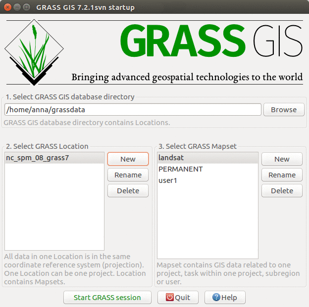
GRASS GIS 7.2 startup dialog with North Carolina sample dataset

Creating new Location and importing data
Although we will spend most of the tutorial working in nc_sm_08_grass7, we will first learn how to create a new Location and import data in there. The CRS will be based on the CRS of the GeoJSON file we downloaded previously. There are other options how to create a new Location, for example by selecting EPSG code, or directly by providing PROJ.4 definition.
In the Welcome screen we click on New in the left part of the screen to launch a Location wizard.
- Type a name of the new Location to Project Location (for example latlon) and press Next
- In our case we select Read projection and datum terms from a georeferenced data file and press Next
- Browse to the downloaded file export.geojson and then press Next
- A summary is shown, press Finish
- It asks whether to import the file, say no.
Now select the new Location and we can see that a PERMANENT Mapset was automatically created. We can start GRASS GIS session. In Layer Manager go to menu File - Import vector data - Simplified vector import with reprojection and select file export.geojson and change the layer name to towers and Import. The points should be automatically added to Map Display.
That's enough for now, we will close GRASS session. When you close GRASS, it asks if you want to close only the GUI or the entire session, because
the GUI is separate from the session. In fact, we can have multiple GUIs running within one session - you launch new GUI instance from running session by typing g.gui from terminal. Running session can be closed by typing exit from your terminal and this launches clean-up procedures.
Now, we will select Quit GRASS GIS.
Note for power users: You can create new Locations from command line, e.g.:
grass -c EPSG:4326 $HOME/grassdata/latlon
Displaying and exploring data
Now we will launch GRASS again in Location nc_spm_08_grass7 in Mapset user1.
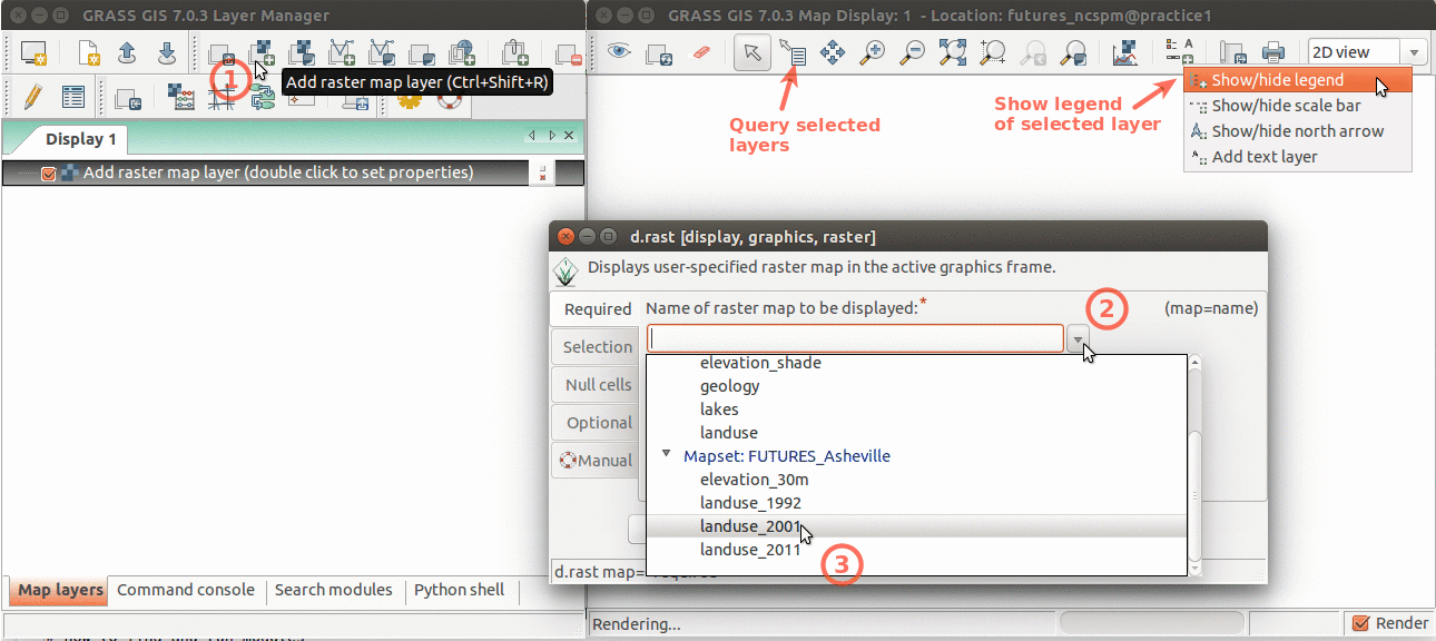
The GUI interface allows you to display raster, vector data as well as navigate through zooming in and out. More advanced exploration and visualization is also possible using, e.g., queries and adding legend. The screenshots below depicts how you can add different map layers (left) and display the metadata of your data layers.
-
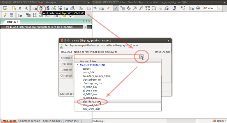
Add raster map layer
-
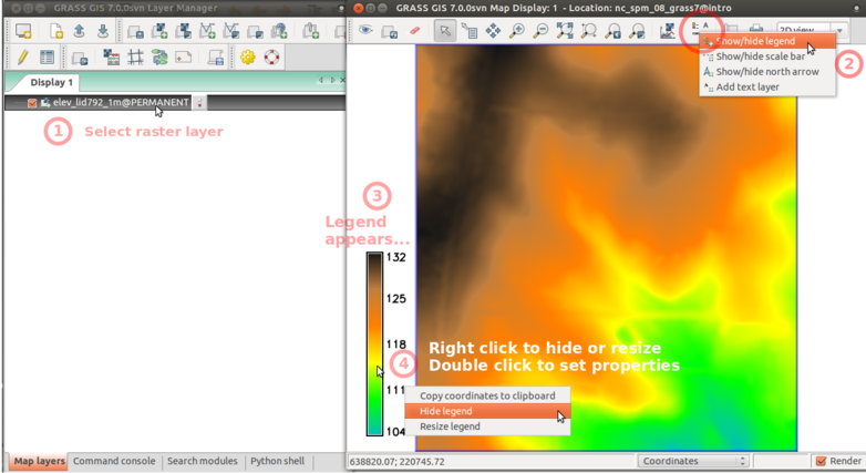
Add raster legend
-
Layer Manager and Map Display overview. Annotations show how to add raster layer, query, add legend.
-
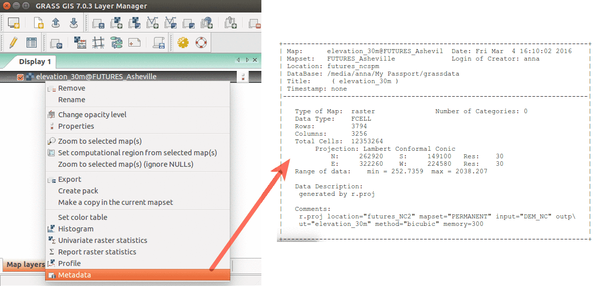
Show raster map metadata by right click on layer


To have a better overview of our raster and vector data, we can use Data tab in Layer Manager. From there we can search for data by name and when we right click at the item, we can select from different actions. In this way we can easily copy or remove data, add them to display, or switch between mapsets. Note that by default for safety reasons you can modify data only in current location and mapset. By unlocking you allow editing other mapsets as well.
-
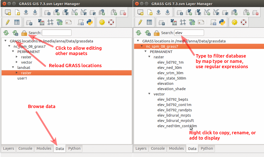
GRASS GIS Data Catalog

GRASS GIS modules
One of the advantages of GRASS is the diversity and number of modules that let you analyze all manner of spatial and temporal. GRASS GIS has over 500 different modules in the core distribution and over 230 addon modules that can be used to prepare and analyze data layers.
GRASS functionality is available through modules (tools, functions). Modules respect the following naming conventions:
| Prefix | Function | Example |
|---|---|---|
| r.* | raster processing | r.mapcalc: map algebra |
| v.* | vector processing | v.clean: topological cleaning |
| i.* | imagery processing | i.segment: object recognition |
| db.* | database management | db.select: select values from table |
| r3.* | 3D raster processing | r3.stats: 3D raster statistics |
| t.* | temporal data processing | t.rast.aggregate: temporal aggregation |
| g.* | general data management | g.rename: renames map |
| d.* | display | d.rast: display raster map |
These are the main groups of modules. There is few more for specific purposes. Note also that some modules have multiple dots in their names. This often suggests further grouping. For example, modules staring with v.net. deal with vector network analysis.
The name of the module helps to understand its function, for example v.in.lidar starts with v so it deals with vector maps, the name follows with in which indicates that the module is for importing the data into GRASS GIS Spatial Database and finally lidar indicates that it deals with lidar point clouds.
Finding and running a module
To find a module for your analysis, type the term into the search box into the Modules tab in the Layer Manager, then keep pressing Enter until you find your module.
Alternatively, you can just browse through the module tree in the Modules tab. You can also browse through the main menu. For example, to find information about a raster map, use: Raster → Reports and statistics → Basic raster metadata.
Advanced search through descriptions, keywords, and optionally manual pages can be performed using the g.search.modules module.
-
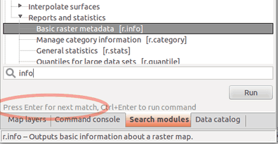
Search for a module in module tree (searches in names, descriptions and keywords)
-
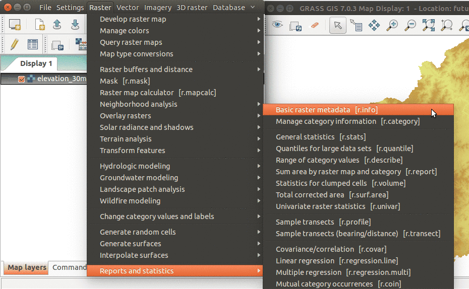
Modules can be also found in the main menu
-
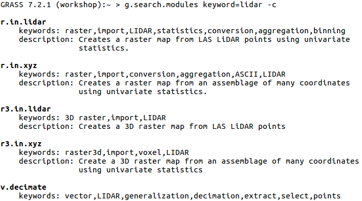
Search for a module using advanced search with g.search.modules


Running a module as a command
If you already know the name of the module, you can just use it in the command line. The GUI offers a Command console tab with command line specifically build for running GRASS GIS modules. If you type module name there, you will get suggestions for automatic completion of the name. After pressing Enter, you will get GUI dialog for the module.
-
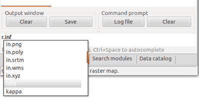
Automatic suggestions when typing name of the module: By typing prefix r. we make a list of modules starting with that prefix to show up.

You can use the command line to run also whole commands for example when you get a command, i.e. module and list of parameters, in the instructions.
Command line vs. GUI interface
GRASS modules can be executed either through a GUI or command line interface. The GUI offers a user-friendly approach to executing modules where the user can navigate to data layers that they would like to analyze and modify processing options with simple check boxes. The GUI also offers an easily accessible manual on how to execute a model. The command line interface allows users to execute a module using command prompts specific to that module. This is handy when you are running similar analyses with minor modification or are familiar with the module commands for quick efficient processing. In this workshop we provide module prompts that can be copied and pasted into the command line for our workflow, but you can use both GUI and command line depending on personal preference. Look how GUI and command line interface represent the same tool.
-

Module dialog

The same analysis can be done using the following command:
v.generalize input=streams@PERMANENT output=streams_generalized method=reumann threshold=10
Conversely, you can fill the GUI dialog parameter by parameter when you have the command.
Computational region
Before we use a module to compute a new raster map, we must set properly computational region. All raster computations will be performed in the specified extent and with the given resolution.
Computational region is an important raster concept in GRASS GIS. In GRASS a computational region can be set, subsetting larger extent data for quicker testing of analysis or analysis of specific regions based on administrative units. We provide a few points to keep in mind when using the computational region function:
- defined by region extent and raster resolution
- applies to all raster operations
- persists between GRASS sessions, can be different for different mapsets
- advantages: keeps your results consistent, avoid clipping, for computationally demanding tasks set region to smaller extent, check your result is good and then set the computational region to the entire study area and rerun analysis
- run
g.region -por in menu Settings - Region - Display region to see current region settings
-
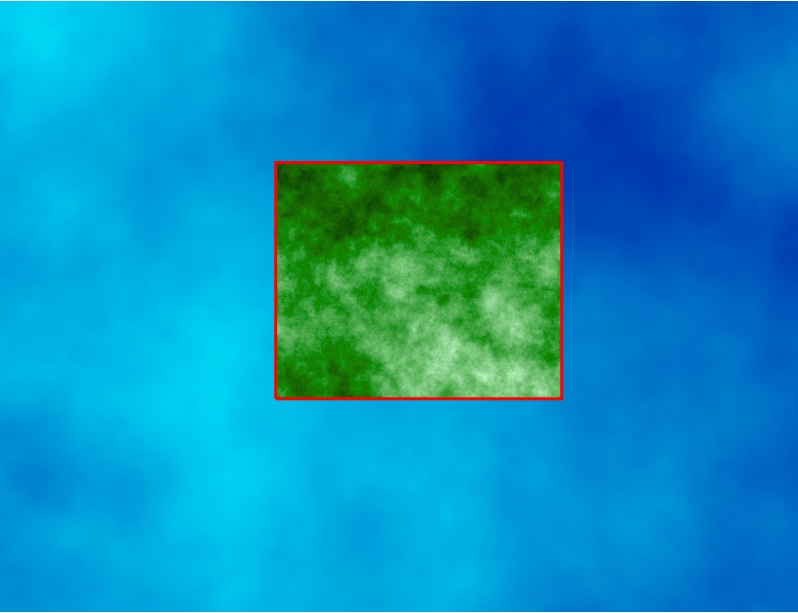
Computational region concept: A raster with large extent (blue) is displayed as well as another raster with smaller extent (green). The computational region (red) is now set to match the smaller raster, so all the computations are limited to the smaller raster extent even if the input is the larger raster. (Not shown on the image: Also the resolution, not only the extent, matches the resolution of the smaller raster.)
-
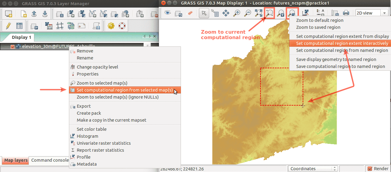
Simple ways to set computational region from GUI. On the left, set region to match raster map. On the right, select the highlighted option and then set region by drawing rectangle.
-
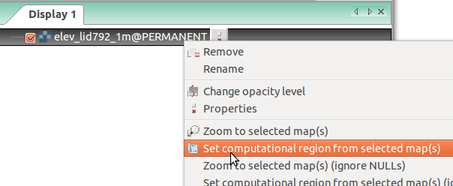
Set computational region (extent and resolution) to match a raster (Layers tab in the Layer Manager)


The numeric values of computational region can be checked using:
g.region -p
After executing the command you will get something like this:
north:      258500
south:      185000
west:       596670
east:       678330
nsres:      10
ewres:      10
rows:       7350
cols:       8166
cells:      60020100
The most common way to set region is based on a raster map - both extent and resolution. If the raster is added to Layer Manager, right click on it and select Set computational region from selected map. Or run the following g.region module (we include -p flag to always see the resulting region):
g.region -p raster=elev_lid792_1m
Computational region can be set also using a vector map, we will use for example elev_lid792_bepts. In that case, only extent is set (as vector map does not have any resolution - at least not in the way raster map does). In GUI, this can be done in the same way as for the raster map. In the command line, it looks like this:
g.region -p vector=elev_lid792_bepts
However now the resolution was adjusted based on the extent of the vector map, it is no longer exact 1m. If that's not desired, we can set it explicitly using -a flag and parameter res. Now the resolution is aligned to even multiples of 1 (the units are the units of the current location, in our case meters):
g.region -p vector=elev_lid792_bepts res=1 -a
Often we need to set computational region based on vector map, but align it with a raster map. For example here we set it based on vector elev_lid792_bepts but align it with raster map elevation:
g.region -p vector=elev_lid792_bepts align=elevation
Running modules
Now let's do some basic raster terrain analysis - computing slope. First set the computational region to match elev_lid792_1m:
g.region raster=elev_lid792_1m
Find the module for computing slope and aspect in menu or the module tree under Raster → Terrain analysis → Slope and aspect or simply run r.slope.aspect.
-
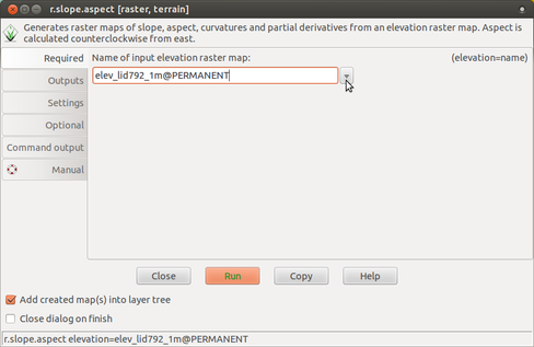
Select input elevation raster map.
-
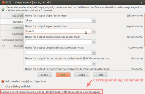
Enter names of output raster maps. Note also the corresponding command at the bottom of the GUI dialog.
-
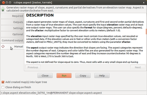
Use manual included in the GUI dialog to refer to details
-
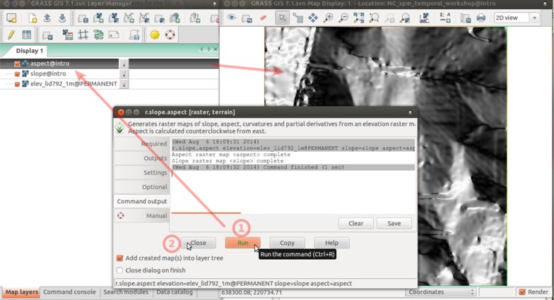
Press Run (1) to compute. When computed result is added to Layer Manager and Map Display. Use Close (2) to close the window.


3D view
We can explore our study area in 3D view.
- Ensure you have elev_lid792_1m added and checked, and then uncheck or remove any other layers. Any checked raster layer will be displayed as a surface.
- Zoom to computational region. Switch to 3D view (in the right corner on Map Display).
- Adjust the view (perspective, height, vertical exaggeration)
- In Data tab, set Fine mode resolution to 1 and set slope (computed in the previous step) as the color of the surface.
- In Appearance tab, adjust light.
- When finished, switch back to 2D view.

Case study part I: basic raster and vector operations
In this exercise we will use viewshed modeling to explore which cell towers (from OpenStreetMap) need to be inspected and then use network analysis to send a cell tower climber to those towers. Then we will analyze which areas need better cell coverage using Python scripting.
You will learn:
- import data
- work with raster and vector modules
- use raster algebra
- run network analysis
- learn basics of Python API
- run Python script
Before proceeding, remove all your layers from Map Display and then add raster elevation and zoom to it.
Data import and reprojection
For this part of our tutorial we need the towers dataset we downloaded in the beginning. Since we have this vector in our newly created Location, we will get it from there. That Location however has different CRS, so we will reproject it with v.proj:
v.proj location=latlon mapset=PERMANENT input=towers
In our case we could also import the original dataset in the same way as before. In menu File - Import vector data select Simplified vector import with reprojection and in the dialog browse to find export.geojson and click button Import. Note that we need to change the output name to towers2. This vector data has different CRS, so a dialog informing you about the need to reproject the data appears and we confirm it.
The imported layer should be added to Map Display, if not, add it manually.
Then select the layer and right click and select Show attribute data to see what kind of attributes there are.
Viewshed modeling
In our (little naive) scenario we investigate which towers stopped working. From our position (632745,224297) we don't receive any signal, so we need to find out which towers are not broadcasting and then go and inspect each of them.
We first compute from which cell towers we should be getting signal by approximating signal propagation by line-of-sight analysis (r.viewshed). Use either the GUI or run the following command from GUI command line:
 g.region raster=elevation -p
 r.viewshed input=elevation output=visible coordinates=632745,224297 target_elevation=50
If we need to rerun the module (for example with different options), we need to check overwrite checkbox, in command line it will look like this:
r.viewshed input=elevation output=visible coordinates=632745,224297 target_elevation=50 --overwrite
Next, we convert the resulting raster representing vertical angle into single-value raster map suitable for conversion to vector using raster algebra. The expression says: create new raster visible_1 where each cell is either 1 or NULL depending on values in raster visible.
r.mapcalc expression="visible_1 = if(visible, 1, null())"
Convert the new raster to vector polygon:
r.to.vect input=visible_1 output=visible type=area
Now we select towers which are inside the area:
v.select ainput=towers atype=point binput=visible btype=area output=visible_towers operator=overlap
The resulting vector has several points as you can check for example in the metadata.
We will add the viewer position into a new vector map and add it to the towers to use it for the network analysis. Module v.in.ascii creates new vector from coordinates provided in a file.
If we run it from GUI dialog of v.in.ascii we can paste the coordinates 632745,224297 into the 'enter values directly' field.
Otherwise we need to create a plain text file with one line having the coordinates. Then we provide the path to that file to v.in.ascii:
v.in.ascii input=path/to/coordinates.txt output=viewpoint separator=comma
Network analysis

Here we show how to do simple network analysis in GUI and what are the actual modules and workflow behind it. First add the following layers (you probably have them already there). You can also paste these individual commands in the GUI command line and press Enter. Don't paste them all at once.
 d.rast map=elevation
 d.vect map=visible color=none fill_color=white width=1
 d.vect map=streets_wake width=1
 d.vect map=viewpoint fill_color=green width=2 icon=basic/marker size=40
 d.vect map=visible_towers fill_color=red width=2 icon=basic/marker size=40
Now select streets_wake in Layer Manager and then go to Map Display - Analyze map - Vector network analysis tool.
- Set Traveling salesman in the top field.
- Go to Parameters tab and make sure you have streets_wake in the first entry.
- Switch tab to Points and click on Add new point so that you have 4 points there (3 points for towers and 1 for viewpoint).
- Click on Insert points from Map Display, select first point and click on Map Display to the place where the viewer is located and then click on each of the visible towers.
- Finally press the top green button to Execute the analysis. Wait for a little bit and then you should be able to see the computed path.
The same can be done using the following module calls.
First create a new vector by merging the visible towers and the viewer position:
v.patch input=visible_towers,viewpoint output=nodes
Then prepare the vector network by inserting new line segments to connect unconnected points to the street network:
v.net input=streets_wake points=nodes output=network operation=connect node_layer=1 threshold=1000
Print the categories of the points in the network map to pass them to the network analysis:
v.category -g input=network type=point option=print
Run the traveling salesman module:
v.net.salesman input=network output=route center_cats=6,7,9,10,11,12,1 node_layer=1
Case study part II: Python scripting
Python intro
The simplest way to execute the Python code which uses GRASS GIS packages is to use Simple Python editor integrated in GRASS GIS (accessible from the toolbar or the Python tab in the Layer Manager). Another option is to write the Python code in your favorite plain text editor like Notepad++ (note that Python editors are plain text editors). Then run the script in GRASS GIS using the main menu File -> Launch script.
-
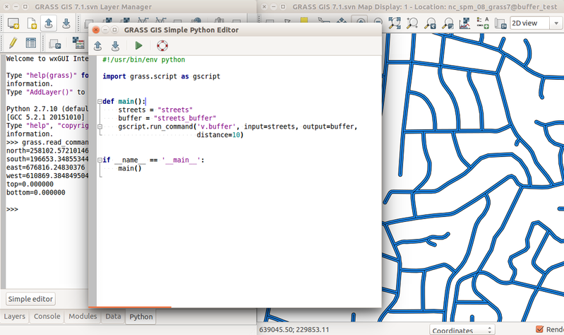
Simple Python Editor integrated in GRASS GIS (since version 7.2) with Python tab in the background which contains an interactive Python shell.
-
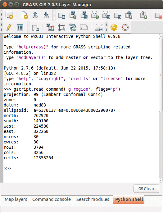
Python tab with an interactive Python shell


The GRASS GIS 7 Python Scripting Library provides functions to call GRASS modules within scripts as subprocesses. The most often used functions include:
- script.core.run_command(): used with modules which output raster/vector data and where text output is not expected or we are not interested in capturing it
- script.core.read_command(): used when we are interested in capturing the text output
- script.core.parse_command(): used with modules producing text output as key=value pair
- script.core.write_command(): for modules expecting text input from either standard input or file
We will use GRASS GUI Simple Python Editor to run the commands. You can open it from Python tab.
For longer scripts, you can create a text file, save it into your current working directory and run it with python myscript.py from the GUI command console or terminal.
When you open Simple Python Editor, you find a short code snippet. It starts with importing GRASS GIS Python Scripting Library:
import grass.script as gs
Note: In certain GRASS GIS versions and code examples, import grass.script as gscript is used.
In the main function, we call g.region to see the current computational region settings:
gs.run_command('g.region', flags='p')
Note that the syntax is similar to bash syntax (g.region -p), only the flag is specified in a parameter. Now we can run the script by pressing the Run button in the toolbar. In Layer Manager we get the output of g.region.
Before running any GRASS raster modules, you need to set the computational region. In this example, we set the computational extent and resolution to the raster layer elevation. Replace the previous g.region command with the following line:
gs.run_command('g.region', raster='elevation')
The run_command() function is the most commonly used one. We will use it to compute viewshed using r.viewshed. Add the following line after g.region command:
gs.run_command('r.viewshed', input='elevation', output='python_viewshed', coordinates=(636054,220707), overwrite=True)
Parameter overwrite is needed if we rerun the script and rewrite the raster.
Now let's look at how big the viewshed is by using
r.univar. Here we use parse_command to obtain the statistics as a Python dictionary
univar = gs.parse_command('r.univar', map='python_viewshed', flags='g')
print(univar['n'])
The printed result is the number of cells of the viewshed.
GRASS GIS Python Scripting Library also provides several wrapper functions for often called modules. List of convenient wrapper functions with examples includes:
- Raster metadata using script.raster.raster_info():
gs.raster_info('python_viewshed') - Vector metadata using script.vector.vector_info():
gs.vector_info('bridges') - List raster data in current location using script.core.list_grouped():
gs.list_grouped(type=['raster']) - Get current computational region using script.core.region():
gs.region()
Here are two commands (to be executed in the Console) often used when working with scripts. First is setting the computational region. We can do that in a script, but it is better and more general to do it before executing the script (so that the script can be used with different computational region settings):
g.region raster=elevation
The second command is handy when we want to run the script again and again. In that case, we first need to remove the created raster maps, for example:
g.remove type=raster pattern="viewshed*"
The above command actually won't remove the maps, but it will inform you which it will remove if you provide the -f flag.
Computing cumulative viewshed

In this exercise we will compute viewshed from each tower using a Python script. From these viewsheds we can then easily compute Cumulative viewshed (in our case meaning from how many towers we get signal at any place). For that we will use module r.series, which overlays the viewshed rasters and computes how many times each cell is visible in all the rasters. This identifies places with bad coverage.
As part of the script we need to create a text file. To ensure the directory is writable, change the current working directory from menu File - Settings - GRASS working environment - Change working directory and select a folder with write permissions.
Copy the following code
into Python Simple Editor (be sure to replace any already existing code) and press Run button.
#!/usr/bin/env python

import grass.script as gs

def main():
    # obtain the coordinates of viewpoints
    viewpoints = gs.read_command('v.out.ascii', input='towers', separator='comma').strip()

    # loop through the viewpoints and compute viewshed from each of them
    for point in viewpoints.splitlines():
        if not point:
            # skip empty lines
            continue
        x, y, cat = point.split(',')
        gs.run_command('r.viewshed', input='elevation', output='viewshed' + cat,
                       coordinates=(x, y), observer_elevation=50, overwrite=True)
    # obtain all viewshed results and set their color to yellow
    # export the list of viewshed map names to a file
    maps_file = 'viewsheds.txt'
    gs.run_command('g.list', type='raster', pattern='viewshed*',
                   output=maps_file, overwrite=True)
    # cumulative viewshed
    gs.run_command('r.series', file=maps_file, output='cumulative_viewshed',
                   method='count', overwrite=True)
    # set color of cumulative viewshed from grey to yellow
    gs.write_command('r.colors', file=maps_file, rules='-',
                     stdin='0% yellow \n 100% yellow')
    gs.write_command('r.colors', map='cumulative_viewshed', rules='-',
                     stdin='0% 70:70:70 \n 100% yellow')

if __name__ == '__main__':
    main()
You can now add all the layers into Map Diplay. Use tool Add multiple raster or vector map layers to add more layers at once, you can filter them by name.
Right click on cumulative_viewshed and select Report raster statistics (r.report) and we can see that almost half of the area has no coverage (we didn't include towers outside of our study area).
Note that there is already addon r.viewshed.cva for computing cumulative viewshed, so we wrote this script for educational purpose.
Try out some of the more advanced and latest features
Hydrology: Estimating inundation extent using HAND methodology
In this example we will use some of GRASS GIS hydrology tools, namely:
- r.watershed: for computing flow accumulation, drainage direction, the location of streams and watershed basins; does not need sink filling because of using least-cost-path to route flow out of sinks
- r.lake: fills a lake to a target water level from a given start point or seed raster
- r.lake.series: addon which runs r.lake for different water levels
- r.stream.distance: for computing the distance to streams or outlet, the relative elevation above streams; the distance and the elevation are calculated along watercourses
r.stream.distance and r.lake.series are addons and we need to install them first:
g.extension r.stream.distance
g.extension r.lake.series
We will estimate inundation extent using Height Above Nearest Drainage methodology (A.D. Nobre, 2011). We will compute HAND terrain model representing the differences in elevation between each grid cell and the elevations of the flowpath-connected downslope grid cell where the flow enters the channel.
First we compute the flow accumulation, drainage and streams (with threshold value of 100000). We convert the streams to vector for better visualization.
g.region raster=elevation -p
r.watershed elevation=elevation accumulation=flowacc drainage=drainage stream=streams threshold=100000
r.to.vect input=streams output=streams type=line
Now we use r.stream.distance with output parameter difference to compute new raster where each cell is the elevation difference between the cell and the the cell on the stream where the cell drains.
r.stream.distance stream_rast=streams direction=drainage elevation=elevation method=downstream difference=above_stream
Before we compute the inundation, we will look at how r.lake works. We compute a lake from specified coordinate and water level:
r.lake elevation=elevation water_level=90 lake=lake coordinates=637877,218475
Now instead of elevation raster we use the HAND raster to simulate 5-meter inundation and as the seed we specify the entire stream.
r.lake elevation=above_stream water_level=5 lake=flood seed=streams
With addon r.lake.series we can create a series of inundation maps with rising water levels:
r.lake.series elevation=above_stream start_water_level=0 end_water_level=5 water_level_step=0.5 output=inundation seed_raster=streams
r.lake.series creates a space-time dataset. We can use temporal modules to further work with the data. for example, we could further compute the volume and extent of flood water using t.rast.univar:
t.rast.univar input=inundation separator=comma
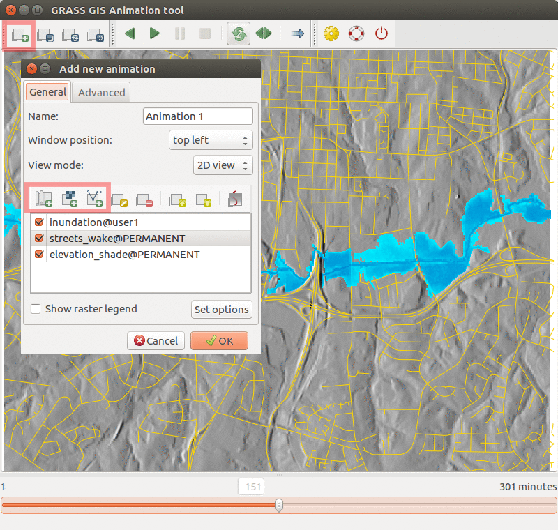
Finally, we can visualize the inundation using Animation Tool.
- Launch it from menu File - Animation tool.
- Start with Add new animation and click on Add space-time dataset or series of map layers.
- In Input data type select Space time raster dataset and below select inundation and press OK.
- Next we want to add shaded relief as base layer. Use Add raster map layer and select raster elevation_shade from mapset PERMANENT.
- You can also overlay road network using Add vector map layer and selecting streets_wake from mapset PERMANENT.
- Select inundation layer and move it above elevation_shade using the toolbar buttons above the layers.
- Press OK and wait till the animation is rendered. Then press Play button.
- Animation tool always renders based on the current computational region. If you want to zoom into a specific area, change the region interactively (see how to do it in the intro), or in command line (e.g.
g.region n=224690 s=221320 w=640120 e=643520) in the Map Display and in Animation tool press Render map
-
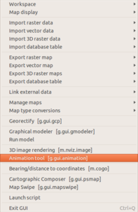
Animation tool in the main menu
-
Inundation computed with r.stream.distance and r.lake.series and visualized in Animation Tool.


Image segmentation

We show two recent segmentation algorithms: i.segment and addon i.superpixels.slic, where the addon needs to be installed first:
g.extension i.superpixels.slic
We show here segmentation of Landsat scene.
Imagery modules typically work with imagery groups. We first list the landsat raster data and then create an imagery group:
g.list type=raster pattern="lsat*" sep=comma mapset=PERMANENT
i.group group=lsat subgroup=lsat input=lsat7_2002_10,lsat7_2002_20,lsat7_2002_30,lsat7_2002_40,lsat7_2002_50,lsat7_2002_61,lsat7_2002_62,lsat7_2002_70,lsat7_2002_80
Now we run i.superpixels.slic and convert the resulting raster to vector for better viewing:
g.region raster=lsat7_2002_10
i.superpixels.slic input=lsat output=superpixels num_pixels=2000
r.to.vect input=superpixels output=superpixels type=area
We do the same for i.segment and convert the resulting raster to vector for better viewing:
i.segment group=lsat output=segments threshold=0.5 minsize=50
r.to.vect input=segments output=segments type=area
From landsat data we also compute NDVI to later display it together with the segmentation:
i.vi red=lsat7_2002_30 output=ndvi viname=ndvi nir=lsat7_2002_40
Remove all layers from Layer Manager and add these layers one by one by pasting into the GUI command line and pressing Enter:
d.rast map=ndvi
d.vect map=superpixels fill_color=none
d.vect map=segments fill_color=none
It's important to note that each segmentation algorithm is designed for different purpose, so we can't directly compare them.
Next steps and alternative workflows can involve: i.segment.hierarchical, i.segment.uspo, i.segment.stats,
r.object.activelearning, r.object.geometry, r.object.spatialautocor.
Batch jobs with --exec
Since GRASS GIS 7.2 modules and scripts can be executed in a GRASS GIS non-interactive session with --exec.
grass path/to/database/location/mapset --exec module params
grass path/to/database/location/mapset --exec script.py params
So for example we can compute viewshed in this way providing we provide correct relative or absolute path to the mapset:
grass grassdata/nc_spm_08_grass7/user1 --exec r.viewshed input=elevation output=viewshed_exec coordinates=642964,222890
This is useful for computing in HPC environments where the processes run in parallel. The individual processes should in general run in different mapsets. If we have an embarrassingly parallel problem we can create a list of these commands, each with different mapset and parameters:
grass -c grassdata/location/mapset_temp_1 --exec python script.py params1
grass -c grassdata/location/mapset_temp_2 --exec python script.py params2
grass -c grassdata/location/mapset_temp_3 --exec python script.py params3
and save them into a text file and use for example GNU Parallel to run them:
parallel --jobs 10 < jobs.txt